|
AltAnalyze Information and
Instructions Version 2.0
Section 1 - Introduction
1.1 Program Description
AltAnalyze (http://altanalyze.org) is a freely available, easy-to-use, cross-platform
application for the end-to-end analysis of microarray, RNA-Seq, proteomic, metabolomic and
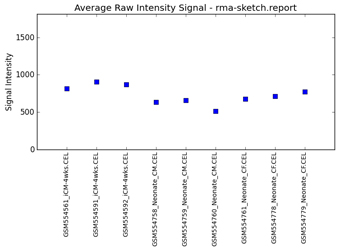
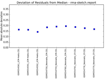
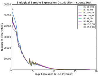
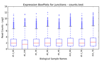
other quantitative datasets. These analyses include QC, gene-expression
summarization, alternative exon/junction
identification, expression clustering, single-cell
analysis, PCA, network analysis, cell type and sample classification,
alternative exon visualization, batch effects removal, ID-mapping, Venn diagram
analysis, pathway/TF target enrichment and pathway visualization. For
splicing-sensitive platforms (RNA-Seq and Affymetrix Exon, Gene and Junction
arrays), AltAnalyze specializes in evaluating changes in protein sequence,
domain composition, and microRNA targeting that result from differential
isoform expression. To do this, AltAnalyze associates user sequence-level
changes in exon or junction expression that lead to the alternative expression
of associated mRNAs. This software requires no advanced knowledge of
bioinformatics programs or scripting. Once
the analysis is complete, a user-friendly Results
Viewer can be run as an independent program or directly from AltAnalyze. As
input from RNA-Seq experiments, AltAnalyze accepts raw RNA sequence files, aligned
BAM files, genomic aligned exons and
junctions from several external packages, or previously normalized expression values. For
Affymetrix analyses, all that is required are your microarray files or a list
of regulated probe sets along with some simple descriptions of the conditions
that you’re analyzing. Step-by-step tutorials are available from our support site
at http://www.altanalyze.org.
AltAnalyze is
composed of a set of modules designed to (A) summarize, organize and filter
exon and junction-level data; (B) annotate and calculate statistics for
differential gene expression, (C) calculate scores for alternative splicing
(AS), alternative promoter selection (APS) or alternative 3’ end-processing;
(D) annotate regulated
alternative exon events (e.g., mutually-exclusive splicing); and (E) assess
downstream predicted functional consequences at the level of protein domains,
microRNA binding sites (miR-BS) and biological pathways. The resulting data
will be a series of text files (results and over-representation analyses) that
you can directly open in a computer spreadsheet program for analysis and
filtering (Figure 1.1). Graphical QC plots, hierarchical clustering heatmaps,
PCA, network diagrams, exon expression graphs and pathway diagrams are also
produced. In addition, export files are created for the Cytoscape
(1)
program DomainGraph to
graphically view domain and miR-BS exon alignments and AltAnalyze statistics, however, these can now also be viewed in AltAnalyze directly through the AltAnalyze Viewer using a new tools called Subgene Viewer.
Alternative exon analysis is
currently compatible with the RNA-Seq unaligned and aligned exon and junction
data, Affymetrix Exon 1.0 ST, Affymetrix Gene 1.0 ST, Affymetrix HJAY, HTA2.0, MJAY,
hGLUE, HTA2.0 arrays and the custom exon-junction Affymetrix AltMouse A array,
however, data from other platforms can be imported if supplied in BED format for over 50 species (Section
1.6). Analysis of these and conventional
Affymetrix microarrays is supported for array normalization (RMA), batch effects removal (combat), calculation of array group
statistics, dataset annotation and pathway over-representation analysis. For
non-Affymetrix arrays, all these steps are supported with exception to array
normalization.
1.2 UpdatesFor past and current updates see: http://code.google.com/p/altanalyze/wiki/News
http://code.google.com/p/altanalyze/wiki/UpdateHistory 1.3 Implementation AltAnalyze is
provided as a stand-alone application that can be run on Windows or Mac OS X
operating systems, without installation of any additional software.
This software is composed of a set of distinct modules written entirely in the
programming language Python and distributed as stand-alone programs and
source-code. Python is a cross-platform
compatible language; therefore, AltAnalyze can be run on any operating system
that has Python and Tkinter for Python installed. On many operating systems,
including Linux and any Mac OS X operating systems the necessary python
components are included by default, however, on some operating systems, such as
Ubuntu, Tkinter may need to be installed when using the graphical user
interface. AltAnalyze can be run from either an intuitive graphic user
interface or from the command-line. Additional source-code dependencies can be
optionally installed to support additional visualization options. To run
AltAnalyze from source-code, rather than through the
compiled executables, see section 1.5 and 2.2 for more information. Note: some features may not be
compatible with all executable operating system versions.
1.4 RequirementsThe basic installation of AltAnalyze requires a minimum of 1GB of hard-drive space for all required databases and components. Species databases are downloaded separately by the user from within the program, for various database versions. Species gene databases, Affymetrix library and annotation files can all be automatically downloaded by AltAnalyze. A minimum of 4GB of RAM and Intel Pentium III processor speed are further required. At least an additional 1GB of free hard-drive space is recommended for building the required output files. Additional RAM (up to 16GB) and hard-drive space (up to 4GB free) is recommended for large exon or junction studies.
1.5 Installation
Prior to downloading AltAnalyze, determine the version that is appropriate to use for your operating system (e.g., Win64 for Windows, OSX for Mac). The operating system specific applications will include all necessary dependencies. If this application fails to run, we recommending downloading the source-code version and installing any necessary dependencies (see below). For RNA-Seq analyses, it is essential to know the genome version your sequences were aligned against and which Ensembl databases support these versions in AltAnalyze. See the Ensembl website (http://ensembl.org) for details.
Compiled Stand-Alone Version Download the installer package (Mac
OS X) or zip archive to your machine. To install on Mac OS X, double-click on
the dmg to mount the AltAnalyze disk image to your Desktop. After opening the
disk image, drag the folder “AltAnalyze” to any desired directory. For zip
archives, extract the archive file to any accessible location using the
appropriate zip extraction tool (e.g., WinZip, default tool). Once extracted,
open the AltAnalyze program directory and double-click on the file named
“AltAnalyze” to start the GUI.
Source-Code Version
When using AltAnalyze in headless
mode (command-line only – Section
2.3), only Python is required (Python 2.6 or 2.7 is recommended). When
using the GUI, both Python and Tkinter are required at a minimum. Tkinter is
typically installed with Python but is not included with some Linux
implementations (e.g., Ubuntu), unless manually installed. Scipy (http://www.scipy.org) is optional
(improves performance when performing a Fisher Exact Test). Numpy (http://www.numpy.org) and
MatPlotLib (http://www.matplotlib.org) are required
for all quality control and clustering analyses and visualization. To support
WikiPathways visualization, install the python web service client package lxml
(http://pypi.python.org/pypi/lxml). If the
Python imaging library Pillow is installed (https://pypi.python.org/pypi/Pillow) direct visualization
of pathways in the GUI is supported as opposed to with the default operating
system PNG image viewer. Additional dependency information and instruction
details can be found here: http://code.google.com/p/altanalyze/wiki/StandAloneDependencies.
Extract the zip archive to any accessible folder. From a command-prompt change directories to the AltAnalyze program folder and enter “python AltAnalyze.py” to initiate the GUI. For headless-mode, supply AltAnalyze with the appropriate command-line arguments (see the end of Section 2 - Running AltAnalyze Locally Using the Command-Line Option). 1.6
Pre-Processing, External Files and Applications
RNA
Sequence Alignment Data
Several
options now exist for importing RNA-Seq data into AltAnalyze, including the
direct alignment of raw RNA-Seq as well as alignment result files. We recommend
reading our online instructions (http://code.google.com/p/altanalyze/wiki/ObtainingRNASeqInputs) to see which
method best suits your data. In general, we recommend TopHat2/BowTie2 as a sensitive method for obtaining known and novel
junctions, in addition to exon-spanning reads.
The
latest versions of AltAnalyze support direct alignment of RNA-Seq fastq or
fastq.gz format files, using the extremely fast and lightweight tool kallisto (http://pachterlab.github.io/kallisto/).
As kallisto’s license has some restrictions, please read before using this
option. Gene and isoform level results are generated from kallisto, but not
exon and junction.
When
analyzing data from already aligned RNA-Seq reads, AltAnalyze can import data
in the BAM alignment file (.bam)
produced by the TopHat or STAR software, UCSC BED format (http://genome.ucsc.edu/FAQ/FAQformat.html#format1), as output
from the Applied Biosystems software BioScope,
or junction expression files supplied by the Cancer Genome Atlas (TCGA). The junction BED file can be
produced by various RNA-Seq exon-exon junction alignment applications,
including TopHat (junction.bed), HMMSplicer (canonical.bed) and SpliceMap
(junction_color.bed). These files provide genomic coordinates and corresponding
aligned read counts for unique junctions. For AltAnalyze, all junction BED
files must be given unique names and saved to a single folder for an experiment
(minimum of two files belonging to two different experimental groups). When
processing BAM files, both junction and exon format BED files will be produced
from each BAM. Upon import, AltAnalyze will match the splice-site coordinates
of each junction to Ensembl and UCSC mRNA annotated exon-junctions, individual
exon splice sites, exons and introns. AltAnalyze will also identify
trans-splicing events, where an aligned junction contains splice sites found
with two distinct genes. If neither splice site of detected junction aligns to
an Ensembl gene (between the 1st and last exons), the junction will
be excluded from the analysis. Junctions and corresponding read counts will be
saved to the folder “ExpressionInput” (user-defined output directory), with
re-assigned standard AltAnalyze IDs (e.g., ENSMUSG00000033871:E13.1-E14.1).
Reciprocal junctions will be analyzed for any known or novel junction predicted
to alternatively regulate an associated exon (see section 3.2 –
Reciprocal Junction Analysis). For SOLiD sequencing, a viable alternative to
these methods is the software BioScope, which produces both exon and junction
expression estimates. The counttag (exon-level) and alternative-splicing
(junction-level) files can be loaded once the extension Is changed from .txt to
.tab. For junction count files from the TCGA,
after downloading to your hard-drive, the extension “.junction_quantification.txt” must be added to all files for
AltAnalyze to recognize the proper input format. AltAnalyze can
process raw Affymetrix image files (CEL files) using the RMA algorithm. This
algorithm is provided through Affymetrix Power Tools (APT) binaries that are
distributed with AltAnalyze in agreement with the GNU distribution license (see
agreement in the AltDatabase/afffymetix/APT directory). Alternatively, users
can pre-process their data outside of AltAnalyze to obtain expression values
using any desired method. Example methods for obtaining such data include
ExpressionConsole (Affymetrix) and R (Bioconductor), either of which can be
used if the user desires another normalization algorithm rather than RMA (e.g.,
GC-RMA, PLIER, dCHIP). Likewise, users with non-Affymetrix data can use an
appropriate normalization method (e.g. http://chipster.csc.fi). FIRMA alternative exon analysis is only supported when users
have previously analyzed CEL files for the dataset of interest, since FIRMA
scores are calculated from RMA probe-level residuals, rather than probe set
expression values.
If
alternative exon, gene or junction Affymetrix CEL files are processed directly
by AltAnalyze (using APT and RMA), two files will be produced; an expression
file (containing probe set and expression values for each array in your study)
and a detection above background (DABG) p-value file (containing corresponding
DABG p-values for each probe set). As
mentioned, if FIRMA is selected as the alternative exon analysis algorithm, APT
will first perform a separate RMA run to produce probe residuals for gene-level
metaprobesets (Ensembl associated AltAnalyze core, extended or full probe
sets). The results produced by AltAnalyze will be identical to those produced
by APT or ExpressionConsole(http://www.affymetrix.com/products/software/specific/expression_console_software.affx). For some
exon arrays, users can choose to exclude certain array probes based on genomic
cross-hybridization (section 2.3).
For array
summarization, all required components are either pre-installed or can be
downloaded by AltAnalyze automatically (Affymetrix library and annotation
files) for most array types. If the user is prompted for a species library file
that cannot be downloaded, the user will be asked to download the appropriate
file from the Affymetrix website. Offline analyses require the user to
follow the instructions in Section 2.3.
Agilent Feature Extraction Files
AltAnalyze directly process Agilent
Feature Extraction files produced from Agilent scanned slide images using
Agilent’s proprietary Feature Extraction Software. Feature Extraction text
files can be loaded in AltAnalyze using the Process Feature Extraction Files option and selecting the appropriate
color ratio or specific color channel from which to extract expression values
from. Quantile normalization is applied by to Agilent data processed through
this workflow.
Other Splicing-Sensitive Platforms
With the
latest version of AltAnalyze (version 2.0.3 and later), any user exon and
junction expression data can be imported into AltAnalyze. This is accomplished
by treating the input expression data the same as the RNA-seq input files
(i.e., stored as junction or exon coordinates and counts in the UCSC BED
format). Analyses, annotations and results are the same as with RNA-seq data.
Example junction BED input: http://code.google.com/p/altanalyze/wiki/JunctionBED
Example
exon BED input: http://code.google.com/p/altanalyze/wiki/ExonBED
Other Quantitative Expression Data
Previously normalized or non-normalized expression values for any experimental data can also be imported into AltAnalyze for analysis. Most analytical functions will be available provided the data is formatted in a compatible manner (e.g., log2, non-zero values). Non-normalized data can be directly normalized in AltAnalyze using the quantile normalization option. When loading gene, protein, RNA or metabolite associated data, biological annotations, pathway enrichment analysis, network visualization and pathway visualization options are also supported. Simply select the Data Type Other IDs from the Main Menu (Section 2.2) and the appropriate identifier system from the platform selection pulldown.
1.7 Help with AltAnalyzeAdditional
documentation, tutorials, help, and user discussions are available at the http://code.google.com/p/altanalyze/wiki/Tutorials. Downloads,
tutorials and help for DomainGraph can be found at http://domaingraph.bioinf.mpi-inf.mpg.de.
Section 2 - Running AltAnalyze2.1 Where to Save Input Expression Files?When
performing analyses in AltAnalyze, the user needs to store all of their
Affymetrix CEL files or sequence alignment count files (BED or TAB) in one directory. This directory can
be placed anywhere on your computer and will be later selected in AltAnalyze. Example files can be downloaded from:
Affymetrix Exon Array
Data BED and TAB Files
http://code.google.com/p/altanalyze/wiki/RNASeq_sample_data
Extract any downloaded
TAR and/or GZIP compressed files prior to analysis.
For Affymetrix array analyses, if
the user has already run normalization on their CEL files outside of AltAnalyze
or have downloaded already analyzed expression data from another source, you can
save the expression and DABG p-value file (optional) anywhere on your computer.
These files should be tab delimited text files that only consist of probe sets,
expression values and headers for each column. Example files can be downloaded http://AltAnalyze.org/normalized_hESC_differentiation.zip.
If
beginning with a tabular expression file, simply save this file to an
accessible file location and create an appropriate output directory, prior to
starting AltAnalyze. If using the command-line for analysis, you will need to
create you groups and comps files prior to calling AltAnalyze as described
here:
http://code.google.com/p/altanalyze/wiki/GroupsAndComps
http://code.google.com/p/altanalyze/wiki/ManualGroupsCompsCreation
2.2 Running AltAnalyze from the Graphic User InterfaceWindows and Mac Directions:
Once you have saved your BAM, FASTQ,
BED, TAB, CEL, TXT or normalized expression value files to a single directory
on your computer, open the AltAnalyze application folder and double-click on
the executable file named “AltAnalyze.exe” (Windows) or “AltAnalyze”
(Mac). This will open a set of user
interface windows where you will be presented with a series of program options
(see following sections). These compiled versions of AltAnalyze can also be run
via a command-line to run remotely or as headless processes (see Section 2.3). Once the analysis is
complete, you can open the other application AltAnalyzeViewer to easily browse your results, rather than
navigate the result files stored on your computer (see the ViewerManual for
details or https://code.google.com/p/altanalyze/wiki/InteractiveResultsViewer).
Unix/Linux and Source Code Directions:
On Linux, download the Linux
executable and python source code archive version of AltAnalyze. To run the
compiled version, double-click the executable file named “AltAnalyze” or open
this file from command-line (./AltAnalyze). These compiled versions of
AltAnalyze can also be run via a command-line to run remotely or as headless
processes (see Section 2.3). If this
file is not compatible with your configuration, you should download the Python
source-code version instead. Start AltAnalyze by opening a terminal window and
changing directories to the AltAnalyze main program (e.g. “cd AltAnalyze_v.2.X.X”
from the program parent directory). Once in this directory, typing “python
AltAnalyze.py” in the terminal window will begin to run AltAnalyze (you should
see the AltAnalyze main menu within a matter of seconds). Prior to running, you
will likely wish to install dependencies required for visualization and
advanced analyses. To do so, see the instructions listed at: http://code.google.com/p/altanalyze/wiki/StandAloneDependencies.
AltAnalyze Graphical Interface Options:
There are many options in
AltAnalyze, which allow the user to customize their output, the types of
analyses they run and the stringency of those analyses. The following sections
show the sequential steps involved in running and navigating AltAnalyze.
Section 2.4 describes each option in detail. Interactive tutorials for
different analyses are provided from the AltAnalyze website. Please note: if you will be using AltAnalyze on a machine
that does NOT have internet access, follow instructions 1-5 below on an online
machine and then copy the AltAnalyze program directory to an offline machine.
1)
Introduction Window – Upon opening AltAnalyze, the user is presented with the AltAnalyze
splash screen and additional information. To directly open the AltAnalyze
download page, follow the hyperlink under “About AltAnalyze”, otherwise select
“Begin Analysis”.
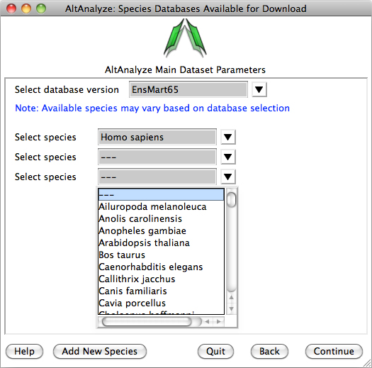
2)
Species Database Installation – The first time AltAnalyze is used, the user will be prompted to
download one or more species database (requires internet connection).
Independent of the data source (e.g., RNASeq or array type) you are analyzing,
select a species and continue. The user can select from different versions of
Ensembl. If your species is not present, select the button Add New Species. Selecting
the option Download/update all gene-set analysis databases will
additionally download GO-Elite annotation databases needed for performing a
wide-array of biological enrichment analyses (pathways, ontologies, TF-targets,
miR-targets, cellular biomarkers) and network visualization analyses.
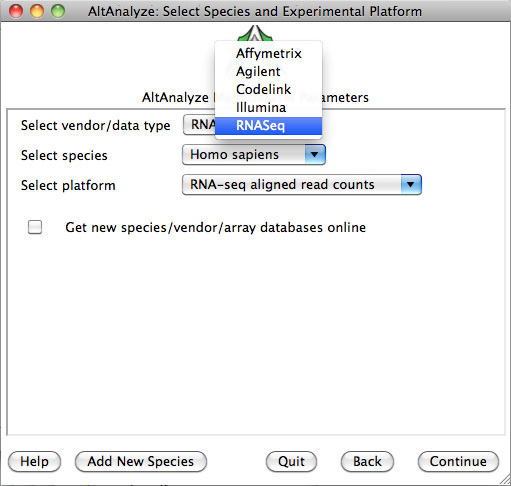
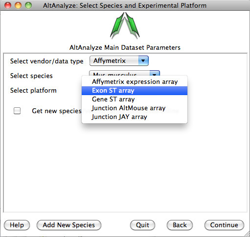
3)
Select species and platform – Next, the user must select a species, array vendor or data type and
platform for analysis (Figure 2.1). Array vendors include Affymetrix, Illumina,
Agilent and Codelink. The data type, Other
ID can be selected if loading non-normalized or normalized values from a
different data source (select ID type under Select Platform). This applies also
to RNA-Seq normalized gene values from a different workflow, such Cufflinks,
eXpress or RSEM. In these cases, match the input ID type (e.g., Symbol,
Ensembl) under Select Platform. If multiple database versions have been
downloaded, the user will also be able to select a version pull-down menu.
After selecting these options click Continue.
4)
Select analysis option–
In this window, the user must select the type data being analyzed. There are four
main types of data; A) FASTQ, BAM, BED, CEL or Feature Extraction files, B)
Expression files (normalized or read counts), C) AltAnalyze filtered files and
D) results from 3rd party applications (Annotate External Results),
E) open the Interactive Results
Viewer or F) perform Additional Analyses.
Processing of CEL files will produce the two file types (expression and DABG),
while processing of BED files will produce a file of exon and/or junction
counts. Processing of Expression files, allows the user to select tab-delimited
text files where the data has already been processed (e.g. RMA or read counts),
which will also produce AltAnalyze filtered files. AltAnalyze filtered files
are written for any splicing array analysis (not for gene expression only
arrays). These later files allow the
user to directly perform splicing analyses, without performing the previous
steps. The AltAnalyze filtered files are stored to the folder “AltExpression”
under the appropriate array and species directories in the user output folder.
Since CEL file normalization and array filtering and summarization can take a
considerable amount of time (depending on the number of arrays), if re-performing
an alternative exon analysis with different parameters, it is recommended that
the user select the Process Expression
file or Process AltAnalyze filtered,
depending on which options the user wants to change. Users can also import
lists of regulated probe sets with statistics obtained from a 3rd party application (e.g., JETTA) other than AltAnalyze using the Annotate External Results option. In
addition, expression clustering, pathway visualization, pathway enrichment and
lineage classification can be independently run on a user expression file using
the option Additional Analyses.
5)
Processing CEL, Feature Extraction or Exon/Junction
Files- If you selected the first option from "Main Dataset Parameters",
you will be presented with a new window for selecting the location of your CEL/FE/BED/TAB
files and desired output directory. Clicking the "select folder" icon
will allow you to browse your hard-drive to select the folder with these data
files. You can double-check the correct directory is selected by looking at the
adjacent text display. For Agilent Feature Extraction files, you will be
presented with the option of selecting which channels or channel ratios to
extract data from. For Affymetrix CEL files, this window will be followed by an
indicator window that will automatically download the library and annotation
files for that array. If the array type is unrecognized and you do not already
have Affymetrix library files for your array (e.g. PGF or CDF), you will need
to download these files from the Affymetrix website. To do so, select the link
at the bottom left side of this window named "Download Library
Files". Select the array type being analyzed from the web page and select
the appropriate library files to download and extract to your computer
(requires an Affymetrix username and password) (Figure 2.3 B). For RNA-Seq
data, the user selects the folder containing their exon and junction input
files in either BED (e.g., TopHat) or TAB (BioScope) files. If the user is
analyzing junction alignment results but does not have exon-level results, the
user can build an annotation file for the program BEDTools, to derive these
results from an available BAM file (e.g., produced by TopHat). To do this, select
the option "Build exon coordinate bed to file obtain BAM file exon
counts". Instead of running the full AltAnalyze pipeline, AltAnalyze will
immediately produce the exon annotation file for BEDTools to the BAMtoBED
folder in the user output directory. Additional details can be found at: http://code.google.com/p/altanalyze/wiki/BAMtoBED.
6)
Summarizing
Gene Data and Filtering For Expression – After obtaining
summary read counts or normalized CEL expression values, a number of options
are available for summarizing gene level expression data, filtering out RNA-Seq
reads and probe sets prior to alternative exon analysis and performing
additional automated analyses (Figure 2.4). Selection of a comparison group
test statistic, allows the user to calculate a p-value for gene expression and
splicing analyses based on different tests (e.g., paired versus unpaired
t-test). Batch-effect correction can be optionally performed with the combat
library (https://github.com/brentp/combat.py).
For applicable platforms, the option to perform quantile normalization is also
provided here. For Affymetrix splicing arrays, AltAnalyze calculates a
“gene-expression” value based on the mean expression of all “core” (Affymetrix
core probe sets and those aligning to known transcript exons) or “constitutive”
(probe sets aligning to those exon regions most common among all transcripts)
probe sets that have a mean DABG p-value less than and a mean expression value
greater the user indicated thresholds for each gene. The same methods are used
for RNA-Seq exon or junction counts, using the same Ensembl and UCSC combined
constitutive evidence. Rather than observed counts, RPKM normalized counts are
selected by default, with counts as an alternative options (Section 3.2). These
values are used to report predicted gene expression changes (independent of
alternative splicing) for all user-defined comparisons (see following section).
In addition, fold changes and ttest p-values are calculated for each of these
group comparisons. These statistics along with several types of gene
annotations exported to a file in the folder “ExpressionOutput” in the
user-defined results directory. Along
with this tab-delimited text file, a similar file with those values most
appropriate for import into the pathway analysis program GenMAPP will also be
produced (Figure 5.1). For splicing analyses, RNA-Seq reads or probe sets with
user defined splicing cutoffs (expression and DABG p-values) will be retained
for further analysis (see section 5.2 – ExpressionBuilder algorithm).
Other analyses, such as QC, PCA, hierarchical clustering (significant genes and
outliers), prediction of which cell lineages are detected and pathway analysis
are also automatically run using these options. If the user selects no for any
these, they can be run again later using the Additional Analyses option from the Select Analysis Method menu.
7)
Select
Alternative Exon Analysis Parameters – If using a junction (RNA-Seq or junction array) or exon-sensitive
array (e.g., Human Affymetrix Exon 1.0 or Gene 1.0
ST), the user will be presented with specific options for that platform (Figure
2.5). These options include alternative exon analysis methods, statistical
thresholds, and options for additional analyses (e.g., MiDAS), however, the
default options are typically recommended. Users can also choose whether to
analyze biological groups as pairwise group comparisons, comparison of all
groups to each other or both. These include combining values for exon-inclusion
junctions and restricting an analysis to a conservative set of Affymetrix probe
sets (e.g., core) and changing the
threshold of splicing statistics. Note: that AltAnalyze’s core includes any probe set associated with a known exon. When
complete, the user can select “Continue” in AltAnalyze to incorporate these
statistics into the analysis.
8)
Assigning
Groups to Samples – When analyzing a dataset for the first
time, the user will need to establish which samples correspond to which groups.
Type in the name of the group adjacent to each sample name from in your dataset
(Figure 2.6 A). When selecting batch-effect correction (combat), an additional menu similar to the group annotation will
appear afterwards asking the user to enter the batch effect for each one. For single-cell datasets or other datasets
where you wish to predict de novo groups, select the Run de novo cluster prediction (ICGS) to discover groups option to
discover clustered sample groups for further analysis in AltAnalyze (See #11
below and Section 3.2 for details.)
9)
Establishing
Comparisons between Groups – Once sample-to-group relationships are
added, the user can list which comparisons they wish to be performed (Figure
2.6 B). For splicing and non-splicing arrays, folds and p-values will be
calculated for each comparison for the gene expression summary file. For
RNA-Seq read or splicing arrays, each comparison will be run in AltAnalyze to
identify alternative exons. Thus, the more pairwise comparisons the longer the
analysis. If the user designates to compare “all groups” and not designate a
pairwise comparison, this window will not be displayed.
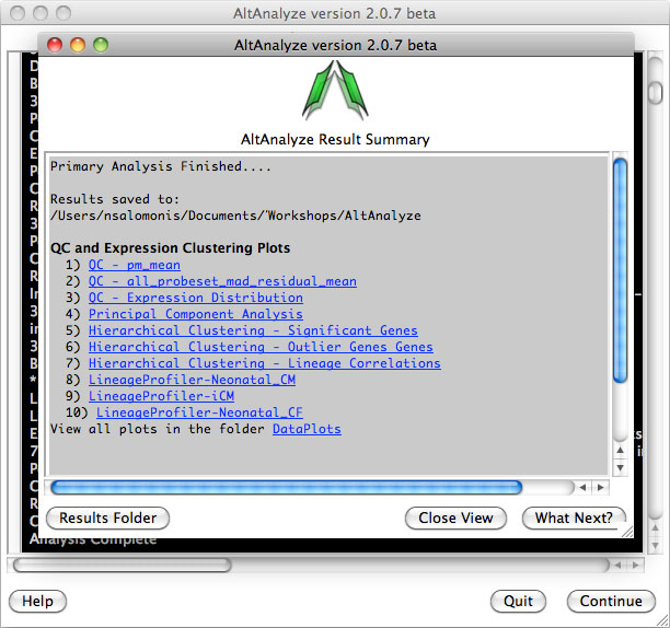
10)
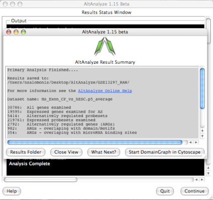
AltAnalyze Status Window -
While the AltAnalyze program is running, several intermediate results files
will be created, including probe set or RNA-Seq read, gene and dataset level
summaries (Section 2.4). The results
window (Figure 2.8) will indicate the progress of each analysis as it is
running. When finished, AltAnalyze will prompt the user that the analysis is
finished and a new “Continue” button will appear. A summary of results appears
containing a basic summary of results from the analysis. This window contains
buttons that will open the folder containing the results and suggestions for
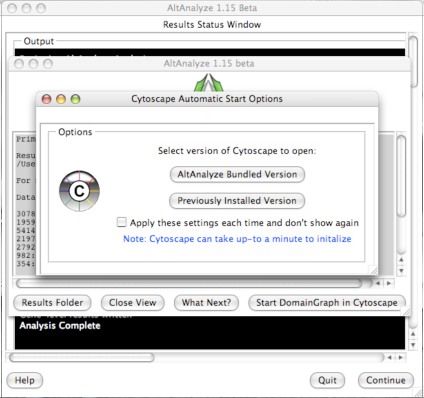
downstream interpretation and analysis. Selecting the button “Start DomainGraph
in Cytoscape” will allow the user to directly open a bundled version of
Cytoscape and DomainGraph (Section 8). In addition to viewing the program
report, this information is written to a time-stamped log text file in the
user-defined output directory.
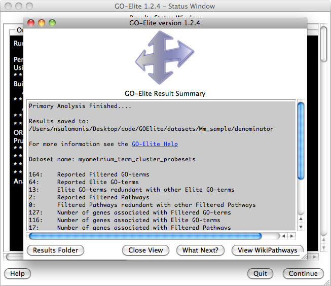
11)
Analyze ontologies and pathways with
GO-Elite – If the
user selects this option during the analysis or following, they will be
presented with a number of options for filtering their expression data to
identify significant regulated genes, perform pathway, ontology or gene-set
over-representation analyses and filter/prune the subsequent results. Selecting
to visualize WikiPathways may significant time to the analysis. Regulated
alternative exons will also be analyzed using GO-Elite. A similar summary results
window as above will also appear with the GO-Elite WikiPathways and Gene
Ontology results (Figure 2.9). For additional information, see: http://genmapp.org/go_elite
12)
Predict Groups from Unknown
Populations (ICGS) – When a priori
sample groups are unknown, such as with Single-Cell
RNA-Seq analyses, it is recommended that the user discover sample groups
clustered based on highly distinct gene or alternative isoform expression
patterns. This can be accomplished by selecting the Run de novo cluster prediction (ICGS) to discover groups option
from the Group selection menu. This menu implements a robust algorithm for
iteratively filtering, correlating and clustering the data to find coherent
gene expression patterns that can inform which sample groups are present. Iterative
Clustering and Guide-gene Selection (ICGS) identifies the predominant
correlated expression patterns from a given gene or splicing dataset to
identify predominant, rare and transitional cell or tissue states. The
resulting menu (Figure 2.10), will
present the user with options for filtering their dataset (RNA-Seq or other
input datasets), based on the maximal non-log expression for each row (Gene TPM
or RPKM filer cutoff), number of associated reads for each gene (if applicable,
otherwise set equal to the above), minimum required fold change difference
between the minimum and maximum expressed samples for each gene and associated
number of samples for this comparison, correlation threshold between genes for
identification of coherent gene set clusters, which features to evaluate (gene,
alternative exons, or both) and which gene sets to optionally build off. Although
designed for RNA-Seq, any datasets can be analyzed with these menu options. The
results will be presented in the form of clustered heatmaps, from which you can
select from different options. Each heatmap will have somewhat distinct sample
clusters from which you can select to perform the conventional AltAnalyze
comparison analysis workflows, using the parameters established in the prior
menu options. As results can vary based on the clustering algorithm used, we
recommend that you have R installed on your computer (not required), to use the
HOPACH clustering algorithm which provides improved results. For Windows
operating systems, R is now included with the binary version of AltAnalyze. Additional
information on ICGS and video tutorials can be found at: http://altanalyze.org/ICGS.html.
AltAnalyze is now
distributed with an integrated application called the AltAnalyze Viewer which
allows uses to immediately and interactively navigate the results from an
AltAnalyze workflow analysis (Section
2.2). This viewer allows the users to navigate all heatmap images,
networks, colored pathways, quality control plots and result tables. In
addition, various interactive plots can be called from this viewer using
built-in AltAnalyze functions, including heatmaps, PCA, SashimiPlots, Domain
and exon expression plots (Figure 2.11).
Tables themselves can be interactively searched for genes and expression data
plotted. An example use of the viewer is shown here: https://www.youtube.com/watch?v=JNA087qBZsc.
Many
of the analysis tools present in AltAnalyze can be run independent of the above
described workflows on user input text files. The input text files are either a
table of log2 expression values, fold-changes or identifiers for
over-representation analysis in GO-Elite. The options are available from the
menu Additional Analyses from the
menu Select Analysis Methods (Figure 2.12) as well as from the
command-line. In addition to the below overviews, more information on these
methods and available options can be found in Section 2.5 and 2.6.
1)
Pathway Enrichment – Performs GO-Elite analysis as described in
the previous section on any existing directory of input and denominator
identifiers. This method runs GO-Elite independent of other AltAnalyze
functions. In addition to saving lists of enriched biological categories, this
tool produced hierarchically clustered heatmaps of enriched terms between input
ID lists along with network graphs displaying interactions between genes and
enriched pathways, ontology terms or gene sets. When the pathway visualization
option is also selected, all enriched WikiPathways will also be exported as
colored PDF and PNG images. If selecting already produced GO-Elite inputs
produced by AltAnalyze, see the folder GO-Elite/input in the AltAnalyze results folder.
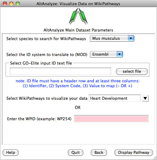
2)
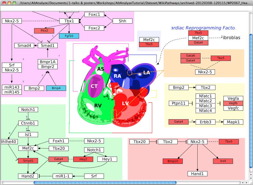
Pathway Visualization – Using the same GO-Elite input files, the
user can select any current WikiPathway and visualize log2 fold changes on the
selected pathway through the AltAnalyze user interface. The input file must
have three columns (ID, SystemCode, FoldChange). Images will be saved as PNG
and PDF files to the same directory as the input file (Figure 2.13). When running from source-code, ensure that the python
packages lxml and requests are installed (Section 1.5).
3)
Hierarchical Clustering – This interface will output a clustered heat
map of rows and columns for any user supplied input text file (Figure 2.14). This file must have
column names (e.g., samples) and row names (e.g., probesets), with the
remaining data as values. The user can choose the clustering algorithm or
metrics to use, whether to cluster rows or columns and what colors to use. This
algorithm is automatically run when using the default AltAnalyze workflows on
two gene-sets: 1) all significantly differentially expressed genes and 2)
outlier regulated genes. These files are available in the folder
ExpressionOutput/Clustering. Significantly differentially expressed genes in
these sets are defined as > 2 fold (up or down) regulated and comparison
statistic p < 0.05 (any comparison), unless the options are changed in the
GO-Elite interface. Outlier genes are those with > 2 fold (up or down)
regulated in any sample relative to the mean expression of all samples for that
gene and not in the significantly differentially expressed list. Many additional advanced
options, including filtering by pathways, ontology terms and
other gene sets and single-cell discovery analysis options are described
in Section 2.6. Resulting clusters are interactive, allowing for viewed
genes to be explored in online databases, pathways to be evaluated for
associated genes and connections and deeper visualization in TreeView by
selection of the TreeView viewer option in the lower left hand corner of the
heatmap. Additionally, visualization of pre-assigned sample groups can be
viewed by adding the group prefix prior to the sample name as a colon separated
annotation (e.g., group_name:sample_name) or analyzing the expression files in
the directory ExpressionInput.
4)
Dimensionality Reduction Analysis – Multiple options
for dimensionality reduction are available in AltAnalyze. These include two and
three-dimensional principal component visualization (using Z-score
normalization) and t-SNE (Figure 2.15).
The top 100 correlated and 100 anti-correlated genes for top 4 PCs (~800 total,
some redundant) with each principal component can be stored by entering a name
for the analysis options menu, for further analysis in the above hierarchical
clustering tool. Additionally, specific genes can be entered into this
interface to color those genes based on their relative expression within the
PCA scatter plot. This analysis is useful for determining how similar samples,
individual cells and biological groups are two each other in the 2D or interactive
3D space (see Section 2.6 for more
details).
5)
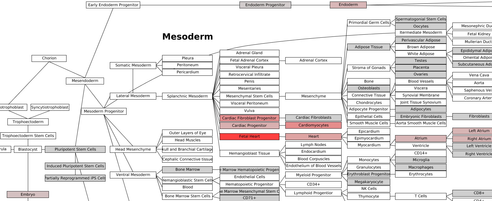
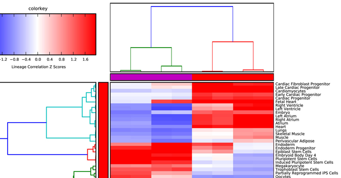
Lineage Analysis – This option allows the user to identify
correlations to over 70 tissues and cell types for a group of biological
sample. The input file must be tab-delimited and have expression values (log2
for microarray datasets) for each array (e.g., probeset) identifier.
Visualization of these results is provided for Z scores calculated from the
lineage correlation coefficients upon a comprehensive Lineage WikiPathways
network and as a hierarchically clustered heat map. Additional options for
alternative modes of sample classification and custom reference sets are
described in Section 2.6.
6)
Network analysis – This option (aka NetPerspective) allows
users to build and view biological interaction networks built using input sets
of genes, protein, metabolite identifiers along with data indicating the
regulation of these genes. See Section
2.6 for more details.
7)
Venn Diagram visualization – To identify the overlap between identifiers
found in two or more files, users can select this menu options to obtain
overlapping Venn Diagrams of the IDs overlapping in distinct files. Two methods
are available for visualization of these diagrams: (A) Standard overlapping
Venn’s and (B) ID membership weighted (See Section
2.6 for more details).
8)
Alternative Exon Visualization – This method allows
users to view either raw exon expression (e.g., RPKMs, probeset intensity) or
gene-normalized normalized expression values (splicing-index) for all
exon-regions for a given set of genes. Users must first select the AltResults
folder from a given experiment. When more than two groups of samples are
present in a given study, it is recommended that the user also perform the
alternative exon anlaysis for all group comparisons (rather than pairwise) to
simultaneously view all biological groups. When viewed in this context,
distinct sample groups are displayed as different colored lines with error bars
indicated by the standard error. Individually entered genes or files containing
many genes can be displayed or saved to the users hard disk (exported to the
folder ExonPlots). For more details,
see Section 2.6.
9)
Identifier Translation – This method can be used to translate from
one gene, protein or metabolite ID system to another. Simply load a file of
interest and select the input ID system and output ID system. A new file will
be saved to the same directory in which the input file is in with the extension
name of the output ID system.
10) Merge Files – This function allows users to identify sets of IDs
that overlap or that are distinct from each other from a set of distinct
files. As many as four files can be
selected, using the options Union or Intersection.
2.3 Running AltAnalyze from Command-LineIn addition to using the
default AltAnalyze graphical user interface (GUI), AltAnalyze can be run by
command line options by calling the python source code in a terminal window or
through other remote services. This option can be used to run AltAnalyze on a
remote server, to batch script AltAnalyze services or avoid having to select
specific options in the GUI. To do this,
the user or program passes specific flags to AltAnalyze to direct it where
files to analyze are, what options to use and where to save results.
Methods for Command-Line Processing
Examples and Flag description
Detailed examples, flag descriptions, default values and associated information can be found at: http://code.google.com/p/altanalyze/wiki/CommandLineMode
Analyzing CEL files –
Affymetrix 3’ array using default options and GO-Elite
python AltAnalyze.py --species Mm --arraytype "3'array" --celdir "C:/CELFiles" --groupdir "C:/CELFiles/groups.CancerCompendium.txt"
--compdir "C:/CELFiles/comps.CancerCompendium.txt"
--output "C:/CELFiles" --expname "CancerCompendium" --runGOElite yes --returnPathways all
Analyzing RNA-Seq (RNASeq) data – BED files using default options
python AltAnalyze.py --species Mm --platform RNASeq --bedDir "C:/BEDFiles" --groupdir "C:/BEDFiles/groups.CancerCompendium.txt" --compdir "C:/BEDFiles/comps.CancerCompendium.txt" --output "C:/BEDFiles" --expname "CancerCompendium"
Analyzing CEL files – Exon
1.0 array using default options
python AltAnalyze.py --species Mm --arraytype exon --celdir "C:/CELFiles" --groupdir "C:/CELFiles/groups.CancerCompendium.txt" --compdir "C:/CELFiles/comps.CancerCompendium.txt" --output "C:/CELFiles" --expname "CancerCompendium" python AltAnalyze.py --species Mm --platform RNASeq –-filterdir "C:/BEDFiles"
--altpermutep 1 --altp 1 --altpermute yes --additionalAlgorithm none --altmethod linearregres --altscore 2 --removeIntronOnlyJunctions yes
Analyzing CEL files – Exon 1.0 array
using custom options
python AltAnalyze.py --species Hs --arraytype exon --celdir "C:/CELFiles" --output "C:/CELFiles" --expname "CancerCompendium" --runGOElite no --dabgp 0.01 --rawexp 100 --avgallss yes ––noxhyb yes --analyzeAllGroups "all groups" ––GEcutoff 4 --probetype core --altp 0.001 --altmethod FIRMA
––altscore 8 --exportnormexp yes ––runMiDAS no --ASfilter yes --mirmethod "two or more" --calcNIp yes
Analyzing CEL files – HJAY
array using custom options
python AltAnalyze.py --species Hs --arraytype junction --celdir "C:/CELFiles"
--output "C:/CELFiles" --expname "CancerCompendium"
--runGOElite no --dabgp 0.01 --rawexp 100 --avgallss yes ––noxhyb yes --analyzeAllGroups "all groups" ––GEcutoff 4 --probetype core --altp 0.001 –altmethod "linearregres"
––altscore 8 --exportnormexp yes ––runMiDAS no --ASfilter yes --mirmethod "two or more" --calcNIp yes --additionalAlgorithm FIRMA ––additionalScore 8
Analyzing Expression file –
Gene 1.0 array using default options, without GO-Elite
python AltAnalyze.py --species Mm --arraytype gene --expdir "C:/CELFiles/ExpressionInput/exp.CancerCompendium.txt" --groupdir "C:/CELFiles/groups.CancerCompendium.txt" --compdir "C:/CELFiles/comps.CancerCompendium.txt" --statdir "C:/CELFiles/ExpressionInput/stats.CancerCompendium.txt" --output
"C:/CELFiles"
Analyzing Filtered Expression file
– Exon 1.0 array using default options
python AltAnalyze.py --species Hs --arraytype exon --filterdir "C:/CELFiles/Filtered/Hs_Exon_prostate_vs_lung.p5_average.txt"
--output "C:/CELFiles"
Annotate External Probe set
results – Exon 1.0 array using default options
python AltAnalyze.py --species Rn --arraytype exon
--annotatedir
"C:/JETTA_Results/Hs_tumor_progression.txt"
--output "C:/JETTA_Results" --runGOElite yes
Filter AltAnalyze results with
predefined IDs using default options
python AltAnalyze.py --species Mm --arraytype gene --celdir "C:/CELFiles" --output "C:/CELFiles" --expname "CancerCompendium" --returnAll yes
Run Lineage Profiler ONLY python AltAnalyze.py --input "/Users/rma/tumors.txt" --runLineageProfiler yes --vendor Affymetrix --platform "3'array" --species Mm
Run Hierarchical Clustering ONLY python AltAnalyze.py --input "/Users/filtered/pluripotency.txt" --image hierarchical --row_method average --column_method single --row_metric cosine --column_metric euclidean --color_gradient red_white_blue --transpose False
Run Principal Component Analysis ONLY AltAnalyze.py --input "/Users/rma/tumors.txt" --image PCA
Return colored WikiPathways ONLY python AltAnalyze.py --input /Users/test/input/differentiation.txt --image WikiPathways --mod Ensembl --species Hs --wpid WP536
Run GO-Elite ONLY python AltAnalyze.py --input "/Mm_sample/input_list_small" --runGOElite yes --denom "/Mm_sample/denominator" –-output "/Mm_sample" --mod Ensembl --species Mm --returnPathways all
(Operating
System Example Folder Locations)
PC: "C:/CELFiles"
Mac
OSX: "/root/user/admin/CELFiles
Linux: "/hd3/home/admin/CELFiles
Primary Analysis Variables
No
default value for these variables is given and must be supplied by the user if
running an analysis. For example, if analyzing CEL files directly in
AltAnalyze, you must include the flags ––species ––arraytype ––celdir ––expname and ––output, with corresponding values.
Likewise, when analyzing an existing expression file you must include the flags ––species ––arraytype ––expdir and ––output.
Most of the variable values are file or folder locations. These variable values
will differ based on the directory path of your files and operating system (e.g, linux has a distinct path
structure than windows – see above examples). The variable name used in
the AltAnalyze source code for each flag is indicated below.
Universally Required Variables
--arraytype: (aka –-platform)
long variable name “array_type”. No default value for
this variable. Options are RNASeq, exon, gene, junction, AltMouse and “3’array”. This variable indicates the
general array type correspond to the input CEL files or expression file. An
example exon array is the Mouse Affymetrix Exon ST 1.0 array, an example gene
array is the Mouse Affymetrix Gene ST 1.0 array and example 3’array is the
Affymetrix Mouse 430 version 2.0 array. See Affymetrix
website for array classifications.
--species:
long variable name “cel_file_dir”. No default value
for this variable. Species codes are provided for this variable (e.g., Hs, Mm, Rn). Additional species can be added through the graphic
user interface.
--output:
long variable name “output_dir”. No default value for
this variable. Required for all analyses. This designates the directory which
results will be saved to.
Analysis Specific Required
Variables
--expname: long variable name “exp_name”. No default value for this variable. Required
when analyzing CEL files. This provides a name for your dataset. This name must
match any existing groups and comps files that already exist. The groups and
comps file indicate which arrays correspond to which biological groups and
which to compare. These files must exist in the designated output directory in
the folder “ExpressionInput” with the names “groups.*expname*.txt” and “comps.*expname*.txt” where expname is
the variable defined in this flag. Alternatively, the user can name their CEL
files such that AltAnalyze can directly determine which group they are (e.g.,
wildtype-1.CEL, cancer-1.CEL, cancer-2.CEL). See http://www.altanalyze.org/manual_groups_comps_creation.htm and http://www.altanalyze.org/automatic_groups_comps_creation.htm for more information
--celdir: (aka --bedDir)
long variable name “cel_file_dir”. No default value
for this variable. Required when analyzing CEL files. This provides the path of
the CEL files to analyze. These must all be in a single folder.
--expdir: long variable name “input_exp_file”. No default value for this variable.
Required when analyzing a processed expression file. This provides the path of
the expression file to analyze.
--statdir: long variable name “input_stats_file”. No default value for this variable. Optional when analyzing a processed expression file. This
provides the path of the DABG p-value file for the designated expression file
to analyze (see –expdir).
--filterdir: long variable name “input_filtered_dir”. No default value for this variable.
Required when aalyzing an AltAnalyze filtered
expression file. This provides the path of the AltAnalyze filtered expression
file to analyze.
--cdfdir: long variable name “input_cdf_file”. No default value for this variable.
Required when directly processing some CEL file types. This variable corresponds to the location of the Affymetrix CDF
or PGF annotation file for the analyzed array. If you are analyzing an exon,
gene, junction, AltMouse or 3’arrays, AltAnalyze has default internet locations
for which to download these files automatically, otherwise, you must download
the compressed CDF file from the Affymetrix website (support), decompress it
(e.g., WinZip) and reference it’s location on your hard-drive using this flag.
If you are unsure whether AltAnalyze can automatically download this file, you
can try to exclude this variable and see if annotations are included in your
gene expression results file.
--csvdir: long variable name “input_annotation_file”. No default value for this variable.
Required when analyzing some expression files or CEL file types. This variable corresponds to the location
of the Affymetrix CSV annotation file for the analyzed array. If you are
analyzing an exon, gene, junction, AltMouse or 3’arrays, AltAnalyze has default
internet locations for which to download these files automatically, otherwise,
you must download the compressed CSV file from the Affymetrix website
(support), decompress it (e.g., WinZip) and reference it’s location on your
hard-drive using this flag. If you are unsure whether AltAnalyze can
automatically download this file, you can try to exclude this variable and see if
annotations are included in your gene expression results file.
--annotatedir: long variable name “external_annotation_dir”. No default value for this
variable. Required when annotating a list regulated probe sets produced outside
of AltAnalyze. This variable corresponds to the location of the directory
containing one or more probe set files. These files can be in the standard
JETTA export format, or otherwise need to have probe set IDs in the first
column. Optionally, these files can have an associated fold change and p-value
(2nd and 3rd columns), which will be reported in the
results file.
--groupdir: long variable name “groups_file”. No default value for this variable. Location of an existing group file to be copied to the directory in
which the expression file is located or will be saved to.
--compdir: long variable name “comps_file”. No default value for this variable. Location
of an existing comps file to be copied to the directory in which the expression
file is located or will be saved to.
Optional Analysis Variables
These
variables are set as to default values when not selected. The default values
are provided in the configurations text file in the Config directory of AltAnalyze (default-**.txt) and can be changed by editing in a
spreadsheet program.
GO-Elite Analysis Variables
AltAnalyze
can optionally subject differentially or alternatively expressed genes
(AltAnalyze and user determined) to an over-representation analysis (ORA) along
Gene Ontology (GO) and pathways (WikiPathways) using the program GO-Elite.
GO-Elite is seamlessly integrated with AltAnalyze and thus can be run using
default parameters either the graphic user interface or command line. To run
GO-Elite using default parameters in command line mode, include the first flag
below with the option yes.
--runGOElite: long variable name “run_GOElite”, default value for this variable: no. Used to indicate whether to run
GO-Elite analysis following AltAnalyze. Indicating yes would prompt GO-Elite to run.
--mod:
long variable name “mod”, default value for this variable: Ensembl. Primary gene system for Gene Ontology (GO) and Pathway
analysis to link Affymetrix probe sets and other output IDs to. Alternative
values: EntrezGene.
--elitepermut: long variable name “goelite_permutations”, default value for this variable: 2000. Number of permutation used by
GO-Elite to calculate an over-representation p-value.
--method:
long variable name “filter_method”, default value for
this variable: z-score. Sorting
method used by GO-Elite to compare and select the top score of related GO
terms. Alternative values: “gene number”
combined
--zscore: long variable name “z_threshold”, default value for this variable: 1.96. Z-score threshold used following
over-representation analysis (ORA) for reported top scoring GO terms and
pathways.
--elitepval: long variable name “p_val_threshold”, default value for this variable: 0.05. Permutation p-value threshold
used ORA analysis for reported top scoring GO terms and pathways.
--dataToAnalyze: long variable name “resources_to_analyze”, default value for this variable: both. Indicates whether to perform ORA
analysis on pathways, Gene Ontology terms or both. Alternative values: Pathways or Gene Ontology
--num:
long variable name “change_threshold”, default value
for this variable: 3. The minimum
number of genes regulated in the input gene list for a GO term or pathway after
ORA, required for GO-Elite reporting.
--GEelitepval:
long variable name “ge_pvalue_cutoffs”, default value
for this variable: 0.05. The minimum
t-test p-value threshold for differentially expressed genes required for
analysis by GO-Elite.
--GEelitefold:
long variable name “ge_fold_cutoffs”, default value
for this variable: 2. The minimum
fold change threshold for differentially expressed genes required for analysis
by GO-Elite. Applied to any group comparisons designated by the user. --additional:
long variable name “additional_resources”, default for this variable: None. When the value is set to one of a valid resource or “all”, GO-Elite will download and incorporate that resource along with the default downloaded (WikiPathways and Gene Ontology). Additional resources currently include the options: “miRNA Targets”, ”GOSlim”, ”Disease Ontology”, ”Phenotype Ontology”, ”KEGG”, “Latest WikiPathways”, ”PathwayCommons”, ”Transcription Factor Targets”, ”Domains” and ”BioMarkers” (include quotes).
--denom:
long variable name “denom_file_dir”, default for this variable: None. This is the folder location containing denominator IDs for corresponding input ID list(s). This variable is only supplied to AltAnalyze when independently using the GO-Elite function to analyze a directory of input IDs (--input) and a corresponding denominator ID list.
--returnPathways:
long variable name “returnPathways”, default for this variable: None. When set equal to “yes” or “all”, will return all WikiPathways as colored PNG or PDF files (by default both) based on the input ID file data and over-representation results. Default value is “None”. When equal to “top5”, GO-Elite will only produce the top 5 (or other user entered number – e.g., top10) ranking WikiPathways.
These
variables are used to determine the format of the expression data being read
into AltAnalyze, the output formats for the resulting gene expression data and
filtering thresholds for expression values prior to alternative exon analysis.
Since AltAnalyze can process both convention (3’array) as well as RNA-Seq data and splicing arrays (exon, gene, junction
or AltMouse), different options are available based on the specific platform.
Universal Array Analysis
Variables
--logexp: long variable name “expression_data_format”, default value for this variable: log for arrays and non-log for RNA-Seq. This is the format of
the input expression data. If analyzing CEL files in AltAnalyze or in running
RMA or GCRMA from another application, the output format of the expression data
is log 2 intensity values. If analyzing MAS5 expression data, this is non-log.
--inclraw: long variable name “include_raw_data”, default value for this variable: yes. When the value of this variable is no, all columns that contain the
expression intensities for individual arrays are excluded from the results
file. The remaining columns are calculated statistics (groups and comparison)
and annotations.
RNASeq, Exon, Gene, Junction or
AltMouse Platform Specific Variables
--dabgp: long variable name “dabg_p”, default value for this variable: 0.05. This p-value corresponds to the
detection above background (DABG) value reported in the “stats.” file from
AltAnalyze, generated along with RMA expression values. A mean p-value for each
probe set for each of the compared biological groups with a value less than
this threshold will be excluded, both biological groups don’t meet this
threshold for a non-constitutive probe set or if one biological group does not
meet this threshold for constitutive probe sets.
--rawexp: long variable name “expression_threshold”, default value for this variable: 70 for microarrays and 2 for RNASeq reads. For Affymetrix arrays, this value is the
non-log RMA average intensity threshold for a biological group required for
inclusion of a probe set. The same rules as the --dabgp apply to this threshold accept
that values below this threshold are excluded when the above rules are not met.
--avgallss: long variable name “avg_all_for_ss”, default value for this variable: no. For RNA-Seq analyses, default is yes. Indicating yes, will force AltAnalyze to use all exon aligning probe sets or
RNA-Seq reads rather than only features that align to predicted constitutive exons
for gene expression determination. This option applies to both the gene
expression export file and to the alternative exon analyses.
--runalt: long variable name “perform_alt_analysis”, default value for this variable: yes. Designating no for this variable will instruct AltAnalyze to only run the gene expression analysis portion of the program, but not the alternative exon analysis portion.
AltAnalyze Alternative Exon Statistics, Filtering and Summarization
Universal Array Analysis
Variables
--altmethod: long variable name “analysis_method”, default value for this variable: splicing-index (exon and gene) and ASPIRE (RNASeq,
junction and AltMouse). For exon, gene and junction arrays, the option FIRMA is also available and for RNASeq, junction and AltMouse platforms the option linearregres is available.
--altp: long variable name “p_threshold”, default value for this variable: 0.05. This variable is the p-value
threshold for reporting alternative exons. This variable applies to both the
MiDAS and splicing-index p-values.
--probetype: long variable name “filter_probe set_types”, default
value for this variable: core (exon
and gene) and all (junction and
AltMouse). This is the class of probe sets to be examined by the alternative
exon analysis. Other options include, extended and full (exon and gene) and “exons-only”, “junctions-only”, “combined-junctions” (RNASeq, junction
and AltMouse).
--altscore: long variable name “alt_exon_fold_variable”, default value for this variable: 2 (splicing-index) and 0.2 (ASPIRE).This is the corresponding
threshold for the default algorithms listed under --altmethod.
--GEcutoff:
long variable name “gene_expression_cutoff”, default
value for this variable: 3. This
value is the non-log gene expression threshold applied to the change in gene
expression (fold) between the two compared biological groups. If a fold change
for a gene is greater than this threshold it is not reported among the results,
since gene expression regulation may interfere with detection of alternative
splicing.
--analyzeAllGroups: long variable name “analyze_all_conditions”, default value for this variable: pairwise. This variable indicates
whether to only perform psiteifalternative exon analyses (between two groups) or to analyze all groups,
without specifying specific comparisons. Other options are “all groups” and both.
--altpermutep: long variable name “permute_p_threshold”, default value for this variable: 0.05. This is the permutation p-value
threshold applied to AltMouse array analyses when generating permutation based
alternative exon p-values. Alternative exon p-values can be applied to either
ASPIRE or linregress analyses.
--altpermute: long variable name “perform_permutation_analysis”, default value for this
variable: yes. This option directs
AltAnalyze to perform the alternative exon p-value analysis for the AltMouse
array (see –altpermutep).
--exportnormexp: long variable name “export_splice_index_values”, default value for this
variable: no. This option directs
AltAnalyze to export the normalized intensity expression values (feature
expression/constitutive expression) for all analyzed features (probe sets or
RNA-Seq reads) rather than perform the typical AltAnalyze analysis when its value
is yes. For junction-sensitive
platforms, rather than exporting the normalized intensities, the ratio of
normalized intensities for the two reciprocal-junctions are exported
(pNI1/pNI2). This step can be useful for analysis of exon array data outside of
AltAnalyze and comparison of alternative exon profiles for many biological
groups (e.g., expression clustering).
--runMiDAS: long variable name “run_MiDAS”, default value for this variable: yes. This option directs AltAnalyze to calculate
and filter alternative exon results based on the MiDAS p-value calculated using
the program Affymetrix Power Tools.
--calcNIp: long variable name “calculate_normIntensity_p”, default value for this
variable: yes. This option directs
AltAnalyze to filter alternative exon results based on the t-test p-value
obtained by comparing either the normalized intensities for the array groups
examined (e.g., control and experimental) (splicing-index) or a t-test p-value
obtained by comparing the FIRMA scores for the arrays in the two compared
groups.
--mirmethod: long variable name “microRNA_prediction_method”, default value for this
variable: one. This option directs
AltAnalyze to return any microRNA binding site predictions (default) or those
that are substantiated by multiple databases (two or more).
--ASfilter:
long variable name “filter_for_AS”, default value for
this variable: no. This option
directs AltAnalyze to only analyze probe sets or RNA-Seq reads for alternative expression that have
an alternative-splicing annotation (e.g., mutually-exclusive, trans-splicing, cassette-exon,
alt-5’, alt-3’, intron-retention), when set equal to yes.
--returnAll: long variable name “return_all”, default value for this variable is no. When set to yes, returns all un-filtered alternative
exon results by setting all associated filtering parameters to the lowest
stringency values. This is equivalent to providing the following flags: --dabgp 1 --rawexp 1 --altp 1 --probetype full --altscore 1 --GEcutoff 10000. Since this option will output all alternative exon scores for all
Ensembl annotated junctions or probe sets, the results file will be exceptionally large (>500,000
lines), unless the user has saved previously run alternative exon results
(e.g., MADS) to the directory “AltDatabase/filtering”
in the AltAnalyze program directory, with a name that matches the analyzed
comparison. For example, if the user has a list of 2,000 MADS regulated probe
sets for cortex versus cerebellum, then the MADS results should be saved to “AltDatabase/filtering” with the name “Cortex_vs_Cerebellum.txt”
and in AltAnalyze the CEL file groups should be named Cortex and Cerebellum and
the comparison should be Cortex versus Cerebellum. When the filename for a file
in the “filtering” directory is contained within the comparison filename
(ignoring “.txt”), only these AltAnalyze IDs or probe sets will be selected
when exporting the results. This analysis will produce a results file with all
AltAnalyze
statistics (default or custom) for
just the selected features, independent of the value of each statistic.
--additionalAlgorithm: long variable name
“additional_algorithms”, default value for this
variable: ‘splicing-index’. For Affymetrix arrays, setting this flag equal to FIRMA changes the individual probe set
analysis algorithm from splicing-index to FIRMA for junction arrays. This
method is applied to RNA-Seq data and junction arrays
following reciprocal-junction analysis (e.g., ASPIRE) in a second run. To
exclude this feature, set variable equal to none.
--additionalScore: long variable name
“additional_score”, default value for this variable: 2. Setting this flag equal to another
numeric value (range 1 to infinity) changes the non-log fold change for the addition_algorithm.
AltAnalyze Database Updates
Universal Array Analysis
Variables
--update:
long variable name “update_method”, default value for
this variable: empty. Setting this
flag equal to Official, without
specifying a version, will download the most up-to-date database for that
species. Other options here are used internally by
AltAnalyze.org for building each new database. See the method “commandLineRun” in AltAnalyze.py for more details.
--version:
long variable name “ensembl_version”, default value
for this variable: current. Setting
this flag equal to a specific Ensembl version name (e.g. EnsMart49) supported by AltAnalyze will download that specific
version for the selected species, while setting this to current will download
the current version.
Additional Analysis, Quality Control and Visualization Options
In addition to the core AltAnalyze workflows (e.g., normalization, gene expression summarization, evaluation of alternative splicing), additional options are available to evaluate the quality of the input data (quality control or QC), evaluate associated cell types and tissues present in each biological sample (Lineage Profiler), cluster samples or genes based on overall similarity (expression clustering) and view regulation data on biological pathways (WikiPathways). These options can be run as apart of the above workflows or often independently using existing AltAnalyze results or input from other programs.
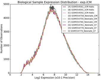
--outputQCPlots:
long variable name “visualize_qc_results”, default value for this variable: yes. Instructs AltAnalyze to calculate
various QC measures specific to the data type analyzed (e.g., exon array,
RNASeq) when a core workflow is run. This will include hierarchical clustering
and PCA plots for genes considered to be differentially expressed (see --GEelitefold and --GEelitepval). Outputs various QC output
plots (PNG and PDF) to the folder “DataPlots” in the user defined output
directory. If run from python source code, requires installation of Scipy,
Numpy and Matplotlib.
--runLineageProfiler:
long variable name “run_lineage_profiler”, default value for this variable: yes. Instructs AltAnalyze to calculate
Pearson correlation coefficients for each analyzed user sample relative to all
cell types and tissues in the BioMarker database. Resulting z-scores for
calculated from the coefficients are automatically visualized on a WikiPathways
Lineage network and are hierarchically clustered. Outputs various tables to the
folder ExpressionOutput and plots (PNG and PDF) to the folder “DataPlots” in the
user defined output directory. Can be run as apart of an existing workflow or
independently with the option --input. If run from python source code, requires
installation of suds, Scipy, Numpy and Matplotlib.
--input:
long variable name “input_file_dir”, default value for this variable: None. Including this option indicates
that the user is referencing an expression file location that is supplied
outside of a normal AltAnalyze workflow. Example analyses include only
performing hierarchical clustering, PCA or GO-Elite.
--image:
long variable name “image_export”, default value for this variable: None. Including this option with any of
the variables: WikiPathways, hierarchical, PCA, along with an input expression file location (--input), will
prompt creation and export of the associated visualization files. These
analyses are outside of the typical AltAnalyze workflows, only requiring the
designated input file. If run from python source code, requires installation of
suds, Scipy, Numpy and Matplotlib.
Hierarchical Clustering Variables
--row_method:
long variable name “row_method”, default value for this variable: average. Indicates the cluster metric
to be applied to rows. Other options include: average, single, complete, weighted
and None. None will result in no row
clustering.
--column_method:
long variable name “column_method”, default value for this variable: single. Indicates the cluster metric to
be applied to columns. These options are the same as row_method.
--row_metric:
long variable name “row_metric”, default value for this variable: cosine. Indicates the cluster distance
metric to be applied to rows. Other options include: braycurtis, canberra,
chebyshev, cityblock, correlation, cosine, dice, euclidean, hamming, jaccard,
kulsinski, mahalanobis, matching, minkowski, rogerstanimoto, russellrao,
seuclidean, sokalmichener, sokalsneath, sqeuclidean and yule (not all may
work). If the input metric fails during the analysis (unknown issue with
Numpy), euclidean will be used instead.
--column_metric:
long variable name “column_metric”, default value for this variable: euclidean. Indicates the cluster
distance metric to be applied to rows. These options are the same as
row_metric.
--color_gradient:
long variable name “image_export”, default value for this variable: red_white_blue. Indicates the color
gradient to be used for visualization as up-null-down. Other options include red_black_sky,
red_black_blue, red_black_green, yellow_black_blue, green_white_purple,
coolwarm and seismic.
--transpose:
long variable name “transpose”, default value for this variable: False. Will transpose the matrix of
columns and rows prior to clustering, when set to True.
2.4 AltAnalyze Analysis OptionsThere
are a number of analysis options provided through the AltAnalyze interface.
This section provides an overview of these options for the different compatible
analyses (gene expression arrays, exon arrays, junction arrays and RNA-Seq
data). For new users, we recommend first running the program with the pre-set defaults
and then modifying the options as necessary.
Selecting the Platform and Species
When
beginning AltAnalyze, the user can select from a variety of species and
platform types. Only array manufacturers and array types supported for each
downloaded species will be displayed along with support for RNA-Seq analysis.
When multiple gene database versions are installed, a drop-down box at the top
of this screen will appear that allows the user to select different gene
database versions. These gene databases include all resources necessary for
gene annotation, alternative exon analysis (where applicable) and Gene Ontology
and pathway analysis. Expression normalization, summarization, annotation and
statistical analysis options are available for all input data types (e.g.,
microarray, RNASeq, proteomics, metabolomics data). At the bottom of this
interface is a check-box that the user can select to download updated species
gene databases, which will bring-up the database downloader window.
Selecting the RNA-Seq Analysis Method
Similar
to microarray analysis options (see below), users can choose to analyze; 1) FASTQ
files (gene expression only), 2) BAM/BED/TAB/TCGA junction files, 3) an already
built RNA-Seq expression file or 4) an AltAnalyze filtered RNA-Seq expression
file for RNA-Seq data.
Option 1 uses the embedded software Kallisto (https://pachterlab.github.io/kallisto/),
which is automatically called to produce pseudoaligned and quantified
transcript expression values from the user supplied single-end or paired-end
FASTQ files. The Kallisto k-mer transcript database is built using annotations
from Ensembl which AltAnalyze downloads automatically, corresponding to the
correct version of the Ensembl (e.g., Ensembl 72). Transcript-level expression
values (TPMs) for mRNAs with experimental evidence are summed at the gene-level
and saved with the prefix exp. to
the folder ExpressionInput. A summary file indicates the estimated read depth
and percentage alignment of each FASTQ pair. Results from this analysis are
immediately processed using the user-defined AltAnalyze workflow options. More
information on this workflow can be found here: https://www.youtube.com/watch?v=Jylu-V7FmpY.
AltAnalyze Since options 3 and 4 produce files from option 2, users will want to begin by
loading a directory of RNA-Seq counts (junction and/or exon) from their
alignment analysis results (BAM files or tabular coordinate result files).
Various programs can be used to produce the BAM or junction .bed format files
that are used as AltAnalyze input. These include HMMSplicer (http://derisilab14.ucsf.edu/software/hmmsplicer/)
and TopHat (http://tophat.cbcb.umd.edu/).
Exon .bed files are produced using BAM files and an AltAnalyze produced input
exon coordinate BED file with BEDTools (http://code.google.com/p/altanalyze/wiki/BAMtoBED). Exon .bed and even junction .bed files are now automatically
generated from supplied BAM files through AltAnalyze rather than deriving these
through BEDTools, although users can still derive these via
BEDTools if they prefer. The junction and exon BED files consist of junction
splice-site coordinates along with the number of reads from a sequencing run
that correspond to that junction.
BED and TAB File Summarization
After
loading junction BED files, AltAnalyze will like link each junction to an
Ensembl gene and known splice-sites based on the provided genomic coordinates.
When novel splice-sites are encountered, AltAnalyze will create a novel
junction annotation for the splice-site (5’ or 3’). In some cases, the
splice-sites may be present in two different genes, indicating trans-splicing.
The number of known-splice sites, novel splice sites and trans-splicing
junctions will be reported upon import and in the log file. The resulting file,
saved to the folder ExpressionInput/exp.NameYouEnter.txt, will contain unique
identifiers indicating the Ensembl gene and associated exon-junction (e.g.,
E13.1-E14.1), indicating the exon block (e.g., “E13”) and exon region (e.g.,
“.1”) that the splice site positions aligns to. When the splice-site is novel
it will be annotated as aligning to the corresponding exon, intron or UTR
region with the additional notation “_position”, where position is the genomic
splice-site coordinate, following the exon region (e.g., E13.1_1000347,
I13.1_1000532, U15.1_1001023). If exon .bed files are present in this same
directory have the same prefix name (e.g., sample1__exon.bed and
sample1__junction.bed), the exon coordinates will be matched to AltAnalyze
annotated exon and intron regions (Ensembl/UCSC) and novel exon regions
inferred from the junction BED locations. Both junction expression and exon
expression will be written to the same file with the prefix “exp.”. This file
can subsequently be loaded as option 2 (“Process Expression File”). The same
process is applied to .tab files from BioScope, accept that exon and junction
count files are produced simultaneously and output to different format files.
Selecting the Microarray Analysis Method
After
the user has selected the species of interest, they must choose what type of
data they will next be analyzing. Data can consist of; 1) Affymetrix CEL files,
2) an already processed expression text files, 3) properly formatted and
filtered AltAnalyze expression input text file or 4) restricted list of probe
sets to be directly analyzed. If beginning with Affymetrix CEL files all three
of these file types are produced in series (see following section) and
automatically processed without any user intervention. If all CEL files from
your study already been previously in AltAnalyze or in another program, the
user can load this file be selecting the option “expression file” and choosing
this text file from your computer. This file needs to contain data from arrays
corresponding to at least two biological groups. Users may wish to re-analyze
these files to change their expression filtering parameters to be more or less
stringent. For the two or more biological groups (see how to define in Figure
2.6), AltAnalyze will segregate the raw data based on the user-defined pairwise
group comparisons and filter the containing probe sets based on whether they
match the user-defined thresholds for inclusion and are associated with Ensembl
genes (see the below section: Expression Analysis Parameters). These files will be saved
to the folder “AltExpression” in the user-defined output directory. These files
can be later selected by choosing the option “AltAnalyze filtered”, if the user
wishes to re-run or use different AltAnalyze alternative exon analysis options
(see below section: Alternative Exon Analysis Parameters).
CEL
files are one of the file types produced after scanning an Affymetrix
microarray. The CEL file is produced automatically from the DAT file (an image
file, similar to a JPEG), by the Affymetrix software by overlaying a grid over
the microarray florescent image and assigning a numeric value to each cell or
probe. From this file, expression values for each probe set can be calculated
and normalized for all arrays in the study using various algorithms.
When choosing to analyze CEL files in AltAnalyze, the user will be
prompted to identify the folder containing the CEL files and the folder in
which to save these other results to. The user will also need to assign a name
to the dataset. These CEL files will be summarized using the RMA algorithm
using the program Affymetrix Power Tools (APT). The APT C++ module
“apt-probeset-summarize” is directly called by AltAnalyze when running
AltAnalyze on a Mac, PC or Linux operating system. Unlike some other
applications, APT is packaged with AltAnalyze and thus does not require
separate installation. However, because it is a separate application there may
be unknown compatibility issues that exist, depending on your specific system
configuration and account privileges. For human and mouse exon arrays,
AltAnalyze also allows for the masking of probes with cross-hybridization
potential, prior to running RMA. This is performed through an experimental APT
function (--kill-list), masking probes that are indicated in files produced for
the MADS application (http://biogibbs.stanford.edu/~yxing/MADS/Annotation.html)
that cross-hybridize to an off-target transcript within 3bp mismatches and a
person correlation coefficient > 0.55, as per the MADS recommendations. The probes with cross-hybridiation potential
are indicated in the AltAnalyze directory “AltDatabase/Hs/exon/Hs_probes_to_remove.txt”.
APT requires the presence of a library file(s) specific for that
array. AltAnalyze will automatically determine the array type and can install
these files if the user wishes (currently most human, rat and mouse arrays
supported). If AltAnalyze does not recognize the specific array type or the
user chooses to download these files themselves, they will need to select the
appropriate files when prompted in AltAnalyze. For exon, gene and junction
arrays, a PGF, CLF and antigenomic BGP file are required. These files will be
automatically downloaded and installed if the user selects “Download” when
prompted. For the AltMouse and 3’arrays, the appropriate CDF file will be
downloaded. In addition to these library files, a NetAffx CSV annotation file
will be downloaded that allows for addition of gene annotations (non-exon
arrays) and Gene Ontology pathway annotations (all arrays). Once installed,
AltAnalyze will recognize these files and automatically use them for all future
analyses. Once the user selects the appropriate directories and files, the user
will be prompted to select the remaining options in AltAnalyze, before APT is
run. Once run, a tab-delimited text
expression file will be produced for all probe sets on the array and a
detection-above background (DABG) p-value file (not applicable to AltMouse or
3’arrays).
Loading a Processed Expression File
If performing an RNA-Seq analysis, this is the file produced immediately after loading and aligning the junctions to exons, introns and UTR regions. For Affymetrix arrays, if CEL files are processed outside of AltAnalyze, the user must save the resulting expression text file in tab-delimited format. It is all right if the first rows in the file have run information as long as they are preceded by a pound sign (#).
Expression Analysis Parameters The
options presented in this interface (Figure 2.4) allow the user to determine
what fields are present in the gene expression output file, what scale the data
is in (e.g. logarithmic), which RNA-Seq reads or probe sets (aka features) to
use when calculating gene expression and how to filter features for subsequent
analyses.
1)
Perform an alternative exon analysis –
Selecting the option “just expression” will halt the analysis after the gene
expression result file has been written, such that no splicing analysis is
performed. This option is only available for splicing-sensitive platforms.
2)
Expression data format –
Indicates the format in which the normalized expression values or counts have
been written. When CEL files have been processed by AltAnalyze,
ExpressionConsole, APT, RMAExpress or through R, the file format will be
logarithmic base 2 (log). The default format of RNA-seq counts is non-log. If
the user designates “non-log”, then expression values will be log base 2 (log2) transformed prior to analysis.
3)
Determine gene expression levels using –
For splicing RNA-Seq and sensitive microarrays, the user has the choice to
alter the way in which gene expression values are calculated and how to filter
their feature-level expression files prior to alternative exon analysis. When
“core” features are selected for this option, all core features (Affymetrix
core annotated and any exon aligning feature) linked to a unique gene will be
used to calculate a measure of gene expression by taking the mean expression of
all associated feature values. When the “constitutive” is selected, only those
features that have been annotated as constitutive or common to the most
isoforms will be used for gene expression calculation. In either case, only features with at least
one array possessing a DABG p-value less than the user threshold (Affymetrix
only) will be retained (if a DABG p-value file is present). In order to exclude
this threshold, set the minimum DABG p-value equal to 1.
4)
Include replicate experimental values in the
export – Instructs AltAnalyze whether to include the expression
values associated with each BED or CEL file in the output file. If not selected
only the mean expression value of all BED or CEL files for each biological
group will be written.
5)
Remove probesets with a DABG p-value above – When a DABG file has been produced (default when summarizing CEL files
with AltAnalyze for exon-arrays), this option is applied. The default DABG
p-value cutoff is p<0.05. This will filter out any non-constitutive probe
set that has a mean DABG p>0.05 for both compared biological groups. For
probe sets used in determining gene expression levels, both biological groups
must have a DABG p < user-value. In order to exclude this option, you can
remove the DABG file (contains the prefix “stats.”), or set this value equal to
1.
6)
Remove probesets/reads expressed below (non-log) – Filters can be applied to both Affymetrix array data and RNA-Seq
datasets to exclude non-expressed probesets, genes, exons or junctions. In all
cases, the expression of a feature is examined (non-log value) to see if that
feature meets the indicated threshold. If not, it is excluded or considered
non-expressed. This can be critical for comparisons where neither condition
demonstrates gene or exon expression and hence can be considered an artifact.
To exclude this option, set the default value to 1 for probeset or read count
thresholds and 0 for RPKM filters.
7)
Comparison group test statistic – Allows the user to calculate a p-value for gene expression and splicing
analyses based on different tests (e.g., paired versus unpaired t-test, rank
sum, Mann Whitney, Kolmogorov Smirnov). These test apply to two sample group
comparisons, whereas any multi-group comparison analyses rely only on an f-test
statistic. For unpaired t-test, the f-test statistic is also used. These tests
are provided through a module of the open-source statistical package Salstat (http://salstat.sourceforge.net/).
8)
Perform expression clustering and visual QC – This option will automatically generate various quality control plots
and hierarchical clustering heatmaps based on the user input dataset analyzed.
Basic quality control metrics include the: 1) distribution of normalized log2
expression values, 2) raw signal intensities (Affymetrix – prior to APT),
3) deviation of residuals from the mean (Affymetrix – post RMA), 4)
Feature-level (exon, junction, intron) expression box-plots (RNA-Seq) and 5)
the total expression of each feature (RNA-Seq) for all analyzed samples.
Principal component analysis and hierarchical clustering are also applied to
all significantly regulated genes (default or user-defined criterion).
Hierarchical clustering is also applied to genes with outlier expression values
to identify poor-replicating samples. When this option is selected, the results
will be available as PDF and PNG in the folder DataPlots and from the GUI once
the analysis is finished (Figure 2.8A). When run from source-code, requires
installation of MatPlotlib and Numpy.
9)
Perform cell profiling with LineageProfiler – Lineage Profiler is a novel tool designed to analyze and visualize the
cellular composition of supplied RNA profiles. Only RNA profiling data with
gene expression values (e.g., Affymetrix and RNA-Seq), as opposed to folds
only, are currently supported. Lineage Profiler produced pearson correlation
coefficients and associated Z scores for each sample analyzed. These Z scores
are visualized as a hierarchically clustered heatmap for all samples and as a comprehensive
lineage network for the biological groups (Figure
2.16). When running from source-code this tool requires the python
libraries lxml, MatPlotLib and Numpy for results visualization and is optimized
to run with Scipy.
10)
Perform ontologies
and pathways with GO-Elite – Choosing “decide later” will allow the
user to view the GO-Elite pathway and Gene Ontology over-representation
analysis options after the main gene expression and/or alternative exon
analysis is run. This will prompt a separate status window and results summary
window displaying over-representation statistics for pathway analysis. If the
option “run immediately” is selected, GO-Elite will run right away without a
separate window. Please note, GO-Elite analysis can take up to an hour per
criterion when using the default parameters, when analyzing all possible
gene-sets, pathways and ontologies. For this reason, multithreading has been
implemented in GO-Elite version 1.2.6 and greater. For more details on this
analysis see: http://www.genmapp.org/go_elite/help_main.htm
Alternative Exon Analysis Parameters
The
options presented in this menu (Figure 2.5) instruct AltAnalyze what
statistical methods to use when determining alternative exon expression, which
features to select for analysis, what domain-level and miR-BS analyses to
perform and what additional values to export for analyses in other tools.
Details on each analysis algorithm are covered in detail in section 3.2.
1)
Select the alternative exon algorithm – For exon and gene arrays, the splicing index and FIRMA methods are
available and for RNA-Seq and junction arrays the ASPIRE and linear regression
methods are available. RNA-Seq and junction analyses can also include single
junction analyses (e.g., Splicing-index, MiDAS), following the reciprocal
junction analysis. These methods are used to calculate an alternative exon
score, relative to gene expression levels. The default value for splicing-index
and FIRMA analyses is 2, indicating that an adjusted expression difference
greater than two fold (up- or down-regulated) is required for the probe set to
be reported. Based on the algorithm, different values and scales will apply.
For junction analyses, the ASPIRE algorithm default cutoff is 0.2, whereas the
linear-regression algorithm is 2. For linear-regression (linearregres), a
minimum value of 2 will select any linear-regression fold greater than 2
(result folds are reported in log 2 scale, however), up- or down-regulated, whereas
ASPIRE’s scores ranging from -1 to 1. See algorithm descriptions for more
details (section 3.2).
2)
Minimum alternative exon score – This value will vary based on the alternative exon analysis method
chosen (see above options).
3)
Max MiDAS/normalized intensity p-value – This is the p-value cutoff applied to MiDAS and splicing-index or FIRMA
ttest p-values for single exon/junction analyses. Currently, the user cannot
set different p-value thresholds for these two statistics. More on MiDAS can be
found below and in section 3.2.
4)
Select probesets to include – This option is used to increase or decrease the stringency of the
analysis. In particular, this option allows the user to restrict what type of
features are to be used to calculate an alternative exon score. In the case of
junction analyses, this option includes the ability to merge the expression
values of junctions/exons that measure the same differential inclusion of an
exon (combined-junctions). For exon and gene arrays, there are three options,
“core”, “extended” and “full”. Although these are the same probe set class
names used by Affymetrix to group probe sets, AltAnalyze uses a modification of
these annotations. Specifically, probe sets with the core annotation include
all Affymetrix core probe sets that specifically overlap with a single Ensembl
gene
(2)
(based on genomic position) along with any
probe set that overlaps with an Ensembl or UCSC exon
(3)
. Likewise, extended
and full probe sets are those remaining probe sets that also align to a single
Ensembl gene, with the Affymetrix extended or full annotation. For RNA-Seq and
junction arrays, options include “all”, “exons-only”, “junctions-only”, “combined-junctions”.
5)
Maximum absolute gene-expression change – This value indicates maximum gene expression fold change (non-log, up-
or down-regulated) that is allowed for a gene to be reported as alternatively
regulated. The default is 3-fold, up or down-regulated. This filter is used
with assumption that alternative splicing is a less critical factor when a gene
is highly differentially expressed.
6)
Perform permutation analysis –
(Junction
Analyses Only) This analysis reports a p-value that represents the
likelihood of the observed alternative exon score occurring by change, after
randomizing the expression values of all samples.
7)
Maximum reciprocal-junction permutatep –
(Junction
Analyses Only) This p-value cutoff applies to the permutation based
alternative exon score p-values when performing ASPIRE or linearregres (see
section 3.2).
8)
Export all normalized intensities – This option can be used to compare alternative exon scores prior to
filtering for biological multiple comparisons, outside of AltAnalyze. For
example, if comparing multiple tissues, the user may wish to export all
normalized intensities (feature non-log expression divided by gene-expression)
for all tissue comparisons. The results will be stored to the AltResults/RawSpliceData
folder in the user-defined output-directory. For junction analyses, the ratio
of the normalized intensities (NI) is reported for the two reciprocal-junctions
(j1 and j2).
9)
Calculate MiDAS p-values – This statistic is analogous to the ttest p-value calculated during the
splicing-index analysis (see section 3.2 for more details). If not selected,
then only the splicing-index or FIRMA (depending on the user selection) fold
and p-value will be used to filter alternative exon results.
10)
Calculate normalized
intensity p-values – Indicates whether to calculate the
splicing-index or FIRMA ttest p-values and filter using the above threshold.
11)
Filter results for
predicted AS – This option instructs AltAnalyze to
only include regulated exons in the output that have been assigned a valid
splicing annotation (e.g., alternative-cassette exon) provided by AltAnalyze.
These annotations exclude exons with no annotations or those with only an
alternative N-terminal exon or alternative promoter annotation.
12)
Align feature to
protein domains using – This option is used to restrict the
annotation source for domain/motif over-representation analysis. If
“direct-alignment” is chosen, only those features that overlap with the genomic
coordinates of a protein domains/motif will be included in the
over-representation analysis, otherwise, the inferred method is used (see
section 3.2 for more details).
13)
Number of algorithms
required for miRNA binding site reporting – This option
is used to filter out miR-BS predictions that only occur in one of the four
miR-BS databases examined. For more miR database information see section 6.5.
14)
Type of group comparison to perform –This option
indicates whether to only perform pairwise alternative exon analyses (between
two groups) or to analyze all groups, without specifying specific comparisons.
2.5 Overview of Analysis ResultsAltAnalyze
will produce three sets of results:
1)
Gene
expression (GE)
2)
Alternative
exon
3)
Diagnostic and
exploratory visualization
These files
are all saved to the user-defined output directory and can be explored through
the use of a spreadsheet data viewer, such as Microsoft Excel or OpenOffice,
and a PDF viewer. Issues reading these
spreadsheets may occur on non-US Windows configurations that (e.g., improper
processing of numbers of with decimals). Additional information on the
statistical methods used and source of annotations can be found in Section 3.
Gene Expression Summary Data
There are five primary GE summary
result files produced by AltAnalyze. These files contain raw data, summary
statistics and/or comprehensive annotations..
1)
DATASET file – Gene
annotations, comparison and ANOVA statistics, raw expression values and counts
(saved to ExpressionOutput).
2)
GenMAPP file –
Comparison statistics (saved to ExpressionOutput).
3)
Summary
statistics file – Overview statistics for protein and non-coding
genes, up- and down-regulated counts and microRNA binding site statistics
(saved to ExpressionOutput).
4)
Clustering
input file – Contains all differentially expressed genes based on user comparisons
(saved to ExpressionOutput/Clustering).
5)
GO-Elite input
files – Lists of differentially expressed genes as input for pathway
over-representation (saved to the folder GO-Elite).
The first is a
file is a complete dataset summary file with the prefix “DATASET-” followed by the user-defined dataset name containing all
array expression values (gene-level for RNA-Seq and tiling-arrays), calculated group statistics (mean expression, folds, raw
and adjusted t-test and f-test p-values) and gene annotations (e.g., gene
symbol, description, Gene Ontology, pathway and some custom groups, genomic
location, protein coding potential, miRNA binding sites). For microRNA arrays,
other annotations from the Affymetrix annotation CSV will replace these (user
supplied). For RNA-Seq and tiling arrays, the
gene expression values are derived from either RNA-Seq reads or probe sets most
informative for transcription (known exons or constitutive) (see “Select
expression analysis parameters”, in Section 2.3). For
RNA-Seq, if only junctions are present, then constitutive junctions or known
junctions will be used, however, if exon reads are present, these will be used
over junction reads. Constitutive features are determined by finding
discrete exon regions that are common to the most mRNA transcripts (Ensembl and
UCSC) for all transcripts used in the AltAnalyze database build (section 6).
For junction arrays (hGlue, HJAY, HTA2.0 and MJAY), both constitutive exon
aligning probe sets and constitutive junction aligning junction probe sets
(most common junctions in mRNAs) are used, whereas for RNA-Seq,
constitutive exons are used. When one or more gene expression reporting probe
sets have DABG p-values with at least one biological group with a mean value
below the user defined threshold, these probe sets will be used to calculate
gene expression, otherwise, all gene expression reporting probe sets will be
used.
The second file, with the prefix “GenMAPP-”, contains a subset of columns
from the dataset summary file for import into GenMAPP
(4)
or PathVisio
(5)
(http://www.pathvisio.org/PathVisio2). This file
has the prefix “GenMAPP” and excludes all gene annotations and individual
sample expression values. This text file can be imported into these programs to
create criterion and color the associated results on pathways (see tutorials
here: http://code.google.com/p/altanalyze/wiki/PathwayAnalysis).
The third
file, with the prefix “SUMMARY-”,
contains overview statistics for that dataset. These results are divided in to
Ensembl protein coding and non-coding genes. Counts for up- and down-regulated
genes are provided separately. Genes called “expressed” are most relevant for
RNA-Seq analyses, where raw counts incremented by 1 for fold calculation
purposes (gene-level). A microRNA count is provided for a single miRNA (miR-1
by default). To change this, users must manually edit the file ExpressionBuilder.py (exportGeneRegulationSummary
function).
The fourth file, with the prefix “SampleLogFolds-“, provides all log2
fold changes relative to the mean expression of all samples in the dataset for
all “regulated” genes. Genes included in this file are those that have greater than 2 fold
(up or down) change in gene expression and comparison statistic p < 0.05 for
any user indicated comparison. To change these defaults, the user must currently
select “run immediately” for the GO-Elite analysis option and change the
associated defaults. This file will be used for (A) hierarchical clustering and
(B) principal component analysis, when these options are selected.
The fifth file type, saved to the
folder “GO-Elite/input” are differentially or alternative expressed genes and
summary statistics for all comparisons. These files are primarily used as input
for performing ontology, pathway or gene-set enrichment analysis using the
GO-Elite option. This analysis can be run along with the default AltAnalyze
workflows, immediately afterwards, or independently using the Additional Analyses menu (Pathway Enrichment option). These lists
can also be used for Pathway
Visualization also from the Additional Analyses menu. These files contain
all differentially expressed genes (prefix GE.),
alternative regulated (prefix AS.),
as well as up and downregulated genes (suffix –upregulated or –downregulated).
The IDs listed will be either the primary microarray identifier or an Ensembl
gene ID, based on the platform analyzed. Also included are the log2-fold
changes and p-values associated with the indicated comparisons. These files may
also be of use in external analysis programs.
Alternative Exon Summary Data
These results are produced from all
features (RNA-Seq reads or probe sets) that may suggest alternative splicing,
alterative promoter regulation, or any other variation relative to the gene
expression for that gene (derived from comparisons file). When the user chooses
to either analyze all groups rather than just pairwise comparisons or both, the
same output files will be produced but report MiDAS p-values comparing all
conditions and the maximum possible splicing index fold between all conditions
(Section 3.2). Each set of results corresponds to a single pairwise comparison
(e.g., cancer vs. normal) and will be named with the group names you assigned.
Four sets of results files are produced in the end:
6)
RNA-Seq or
probe set-level – Feature-level statistics, exon annotations, AS/APS
annotations, and functional predictions (protein, domain and miRNA binding
site).
7)
Gene-level –
Gene-level summary of data in feature-level file.
8)
Domain-level –
Over-representation analysis of gene-level domain changes due alternative exon
regulation.
9)
miRNA binding
sites – Over-representation analysis of gene-level, predicted miRNA binding
sites present in alternatively regulation exons.
10)
DomainGraph input file –
Direct or inferred Affymetrix Exon 1.0 ST probe set IDs and summary statistics
(see file #4) for analysis in DomainGraph. For non-exon arrays (e.g., RNA-Seq,
Affymetrix junction or gene arrays), corresponding regulated exons are
translated to the overlapping exon ID (see Section 8).
11)
All processed splicing scores –
Feature-level statistics (see file #4) above for all analyzed features (not
just significant). This is in the same format as the DomainGraph export file
(see file #7).
12)
All feature-normalized intensities–
(optional) Feature-level normalized intensities (see file #4) used to calculate
splicing-index statistics or FIRMA fold changes for each sample. To obtain this
file “Export all normalized intensities” option.
13)
Summary statistics file –
Global statistics, reporting the number of genes alternatively regulated,
number differentially expressed and summary protein association information
(e.g., mean regulated protein length).
Each
file is a tab delimited text file that can be opened, sorted and filtered in a
spreadsheet program. These files are
saved to the user-defined output directory under “AltResults/AlternativeOutput”, all with the same prefix (pairwise
group comparisons). AltAnalyze will analyze all pairwise comparisons in
succession and combine the feature-level and gene-level results into two
additional separate files (named based on the splicing algorithm chosen).
Feature- and
Gene-Level Alternative Exon Result Files
The
feature-level file contains alternative exon data for either one probe set
(exon-array), exon/junction IDs or reciprocal junctions (RNA-Seq and junction arrays). More information on
these fields can be found at http://code.google.com/p/altanalyze/wiki/ProteinDirectionIndicator. In general,
these file include:
The gene-level
file contains a summary of the data at the gene level, with each row
representing a unique gene. This file
also includes:
·
Gene Ontology and pathway information for each gene obtained
from Ensembl.
Protein Domain/Motif
and miRNA Binding Site Over Representation Files
Over-representation
analyses, (files 3 and 4) have the same structure:
Comparison
Evidence File
A common
question for biologists analyzing alternative exon profiles is which events are
most likely true versus false positive predictions. RNA-Seq and junction
microarrays allow for independent detection of alternative splicing events
using only exon-junctions or only detected exons. The comparison evidence file
examines results from the reciprocal junction analysis (ASPIRE or Linear
Regression) and the single feature (exon or junction) analysis
(splicing-index), to determine which events are predicted by both analyses or
only be one. Those splicing-events predicted by both represented independently
verified events that are most likely to represent valid known or novel
alternative splicing events in the dataset. This file includes:
Diagnostic and Exploratory Visualization Results
In addition to
the results files listed in the previous sections, various image plots are
produced by AltAnalyze to assess quality control (QC), cluster gene or sample
profiles (clustering) and identify associated cell types represented in each
sample (Lineage Profiler). All plots are saved to the folder DataPlots in the user-defined output
directory. Unlike the other AltAnalyze methods, these analyses require the
installation of non-default Python packages if running directly from the Python
source-code (see Section 1.5). However, these dependencies are already included
in the OS specific binary distributions.
Basic Quality
Control
Multiple basic
quality control plots are produced by AltAnalyze to evaluate sample quality and
overall technical similarity to other samples in the dataset. Different QC metrics are applied based on
whether the input data is from: (A) AltAnalyze normalized Affymetrix files, (B)
RNA-Seq data or (C) pre-processed expression files.
If
data from (A) applies, three output QC files will be generated: 1) distribution
of normalized log2 probeset intensity values, 2) mean raw signal intensities of
each array and 3) mean absolute deviation (MAD) of the RMA residuals for each
array (Figure 2.17 A-C). The source
data for all of these three QC metrics are derived from Affymetrix Power Tools
(Section 1.6) RMA analysis built into AltAnalyze. For more details see: http://bib.oxfordjournals.org/content/early/2011/04/15/bib.bbq086.full.
If data from (B) applies, three
groups of QC files will be generated: 1) distribution of log2 read-counts (exon
and junction), 2) feature-level box-plots for the distribution of exon,
junction and intron read-counts and 3) total number of reads for each sample,
broken down by exon, junction and intron aligning (Figure 2.17 D-F). This source data for these plots is obtained from
the file with the prefix counts in the folder ExpressionInput, which includes where each feature aligns to and
the total number of associated read counts.
Data
from © consist only of the distribution of log2 values in the input file.
Expression Clustering
Two main
expression clustering methods are currently output by AltAnalyze, hierarchical
clustering and principal component analysis (PCA). Hierarchical clustering is used to identify
overall patterns of gene expression shared by groups of genes and samples
whereas PCA is used to visualize similarities between samples within and
between groups in 2D dimension space. Hence, both methods can be used to
evaluate the quality of the data as well as explore sample or gene
relationships.
Hierarchical
clustering is applied by default to both significantly differentially expressed
genes and outlier regulated genes from the entire dataset. Genes considered
significantly regulated are those that have greater than 2 fold (up or down) change in gene
expression and comparison statistic p < 0.05 for any user indicated
comparison (see GO-Elite options for details on changing the defaults –
Figure 2.9). Outlier genes are those with a greater than 2 fold difference
relative to the mean of all samples, for any gene not in the significantly
regulated set. For significantly regulated genes, sample folds are calculated
as compared to the mean of all samples for each gene or based on the group
comparisons designated by the user (called “Relative”). Although default
clustering metrics, methods and coloring options are applied to the resulting
heatmaps, these options can be changed after running AltAnalyze (see Additional Analyses – Section
2.2). Vector based versions of these plots are available in the PDF outputs in
the folder DataPlots. A text file
representing the clustered matrix, identifiers and flat-clusters will be
exported to the DataPlots directory
along with a TreeView compatible .cdt file. Note: Only row names are
included when the number of rows visualized is less than 100. Clustering is
accomplished using Scipy’s cluster.hierarchy method. For additional details and
workflows, see associated online Tutorials: https://code.google.com/p/altanalyze/wiki/Tutorials.
PCA is
applied only to the significantly differentially regulated gene set, by
default. In this plot, the values of 1st component are plotted
against the values of the second component for each sample (Figure 2.15). This analysis will
visualize each sample as a colored circle, with the color corresponding to the
different assigned biological groups. The sample names will be displayed to the
right of the sample circle.
Lineage
Profiler Analysis
Lineage
Profiler is a new method introduced in AltAnalyze version 2.07. This algorithm
correlates user supplied sample expression profiles with previously collected
expression profiles from a large compendium of publically available cell types
and tissues (aka lineages). The underlying lineage data is biased towards
adult, fetal and progenitor cell types arising throughout differentiation, as
opposed to disease states or cell lines. It is capable of characterizing both
microarray and RNA-Seq datasets for a diverse database of cell lineages.
The
compendium itself is built on top of either exon or 3’array publically
available datasets (human and mouse) combined from a large number of studies.
From the entire compendium dataset, only the top 60 cell-specific markers are
used for the lineage correlation analysis (see AltDatabase/EnsMart65/uclidea/Hs/Hs_exon_tissue-specific_protein_coding.txt).
The top markers are selected during the LineageProfiler database build process,
based on their overall expression correlation to a specific-cell type relative
to all other cell types examined. Additional details on the LineageProfiler algorithm can be found at http://code.google.com/p/altanalyze/wiki/LineageProfiler.
Three
main output files are currently provided by LineageProfiler: (1) sample-to-cell
type correlation statistic flat-files, (2) hierarchically clustered heatmap of
correlation statistics and (3) visualization of the correlation statics along a
comprehensive lineage network. The primary statistic used form these analyses
is a Z score calculated from the distribution of Pearson correlation
coefficients for each user supplied RNA-profile to all analyzed lineages.
The
correlation statistics flat-files are produced by LineageProfiler: (A)
Pearson-correlation coefficients (ExpressionOutput/LineageCorrelations-<dataset_name>.txt), (B) derived
Z scores (ExpressionOutput/LineageCorrelations-<dataset_name>-zscores.txt) and (C) average Z scores for each
biological group (ExpressionOutput/Clustering/LineageCorrelations-<dataset_name>-zscores-groups.txt).
These files are all tab-delimited text files that can be easily explored in a
spreadsheet viewer, such as Excel.
The
hierarchically clustered heatmap output (2) is based on file (B). An example of
this output is shown in Figure 2.16B.
This output is particularly useful for identifying changes in lineage
associations during developmental transitions.
To further understand which cell fate decisions or
lineage pathways are regulated in particular biological conditions,
visualization along a comprehensive lineage network is provided (3) derived
from file ©. An example of this output is shown in Figure 2.16A. The lineage network is a community curated network
posted at WikiPathways (http://wikipathways.org/index.php/Pathway:WP2062).
This network is visualized using the WikiPathways API (Wikipathways_webservice.py
> viewLineageProfilerResults()). When running AltAnalyze from source-code, this function
requires installation of the lxml library.
2.6 Additional à la carte AnalysesIn addition to the
streamlined AltAnalyze pipeline analyses, a number of individual useful
functions can be run independently of these workflows. These include:
These functions provide a
wide array of solutions for genomics analysis that are easily accessible to
bioinformaticians and experimental biologists alike. These functions can be
accessed through the Additional Analyses menu after selecting a species and
platform type in the main menu. Alternatively, the functions can be run from
the command-line for batch customized analytical and batch pipelines (see
Section 2.4).
Pathway Analysis and Visualization
Pathway enrichment and visualization
methods are identical to those provided in the independent analysis package
GO-Elite. Enrichment analysis is available using a multiple algorithms, user
defined thresholds and can be run on over a dozen distinct biological gene and
metabolite categories. This tool provides an optimized list of enriched
biological categories (e.g., Ontology term pruning) for description of input ID
lists. In addition to tabular result files, hierarchically clustered heatmaps are
displayed showing enrichment of terms between distinct conditions analyzed as
well as networks of enriched terms with corresponding regulated genes. For more
details see http://genmapp.org/go_elite/help_main.htm.
Hierarchical Clustering and Visualization
AltAnalyze can perform
hierarchical clustering using default options (see Section 2.5 –
Expression Clustering) or using customized options. These include the ability
to change visualization modes (e.g., colors, contrast), clustering algorithm
(e.g., cosine, uclidean, hopach), row normalization, matrix transposition and
biological group coloring. In addition, several advanced options are available
including the ability to cluster and visualize genes associated with certain
GO-Elite pathways, ontologies or gene-sets and obtaining clusters of genes most
correlated with a single candidate. These advanced options allow any users to
easily and quickly obtain highly specialized expression views using a large
selection set of biological categories, visualization options and advanced
clustering algorithms from a single interface (Figure 2.17A). More details on
these options and parameters are described at http://code.google.com/p/altanalyze/wiki/Heatmaps.
Principal Component Analysis (PCA)
In addition to the default
pipeline output of two-dimension PCA plots (first two components – see
Section 2.5), PCA can be run on its own using multiple customized options.
These include optionally displaying sample labels and viewing a PCA plot interactively
in three-dimensions as shown in Figure 2.17B. The percentage of variance
explained for each component is annotated in the component label. The top
correlated and anti-correlated genes associated with the top four principal
components are stored in the folder DataPlots/PCA.txt and can optionally be
stored as an available gene set for other downstream analyses by entering a name
for the analysis in the GUI.
Lineage Analysis and Sample Classification
This menu provides a number
of flexible options for classifying samples relative to either (A) pre-compiled
tissue/cell type references built from various transcriptome measurement platforms
or (B) relative to a user supplied set of reference measurements. For tissue
and cell-type classification, the LineageProfiler algorithm is employed, in
which each loaded sample is matched to a set of tissue-specific markers
determined from AltAnalyze’s MarkerFinder algorithm and then correlated to all
available compendium cell type or tissue expression values. Although the
overall correlation (Pearson correlation coefficient) between distinct
platforms may be low (e.g., RNA-Seq versus exon array profiles), these sample
specific correlations most typically are accurate, especially where many
distinct sample types are being compared (manuscript in preparation). Results
are output as a lineage correlation heatmap and as a WikiPathway network for
lineage differentiation (DataPlots folder). The results in these files are z-scores derived from the distribution
of observed correlations for all samples analyzed in a given experiment.
In addition to lineage classification, this algorithm can
be applied to custom references and even distinct gene-models, discovered using
the LineageProfilerIterate.py script provided with AltAnalyze. Using this
method, samples can be classified using user-supplied references for all
analyzed genes or subsets of gene-models provided in a gene-model file.
Additional information on these methods, example workflows and example files
are provided online at:
http://code.google.com/p/altanalyze/wiki/LineageProfiler
http://code.google.com/p/altanalyze/wiki/SampleClassification
Network Analysis and Visualization (NetPerspective)
NetPerspective is a new
tool introduced in AltAnalyze 2.0.8 that allows users to quickly and easily
identify hypothetical biological networks between interacting genes, proteins,
RNAs and metabolites with a single query. NetPerspective uses a collection of
highly curated interactions from WikiPathways, KEGG and HMDB, experimentally
derived transcription factor targets, annotated drug-protein interactions,
microRNA target predictions (Section 3.7) and speculative protein interactions
from BioGRID. Networks can be generated from lists of input IDs, existing
interactions or GO-Elite pathways/gene-sets/ontologies, visualized with
regulated gene, proteins and metabolites. Connections between sets of IDs can
be identified using direct interactions, indirect or from the shortest path of
possible connections. These networks are automatically displayed when run from
the GUI and are also saved as PDF and PNG files to the folder network in the input file directory
(Figure 2.19). When run from the command-line, automated generation of networks
and images can be performed for an unlimited number of input lists run
sequentially or in parallel. More details on these options and parameters are
described at http://code.google.com/p/altanalyze/wiki/NetPerspective.
Alternative Exon Visualization (AltExonViewer)
An important means for
initial validation of alternative exon expression (e.g., alternative splicing,
alternative promoter regulation) is visualization of feature expression in the
context of all measured gene features. In addition to visualization of
alternative exons in the Cytoscape plugin DomainGraph (Section 8), AltAnalyze contains a built in alternative exon viewer
called AltExonViewer. This function allows users to display gene data in the
form of a 1) line graph depicting exons
along the X-axis and exon-expression or splicing index fold change along the
Y-axis, 2) a heatmap of all exons
across all samples and 3) a Sashimi-Plot genomic view. For the line graph option,
expression values from each group are summarized as a single line color, with
standard-error values included. One gene or multiple genes can be displayed at
a time using a manual text entry field (e.g., SOX2 NANOG POU5F1 TCF7L1) or
through a file selection option. Probed UTR regions and Introns can also be
optionally displayed. To visualize exon-expression, select the raw expression option. This option
requires that input expression files have already been generated and analyzed
with AltAnalyze (conforming to the standard file locations – e.g.,
ExpressionInput/exp. File). To visualize alternative exon-expression directly,
select the splicing-index option.
This option works for already produced alternative exon results, which are
saved to the folder AltResults/RawSpliceData (Figure 2.20). When analyzing a dataset with more than two groups,
re-run the AltAnalyze workflow beginning with the Process AltAnalyze Filtered
option and selecting the all groups selection
for Comparisons to Perform option.
For the heatmap view, a standard AltAnalyze
heatmap is produced with all exon region expression values (median normalized),
ordered from beginning to end along the y-axis. The Sashimi-Plot option,
directly interfaces with the Sashimi-Plot source python code (http://miso.readthedocs.org/en/latest/sashimi.html),
to produce high resolution splicing plots. Additional details on these options and parameters are described at http://code.google.com/p/altanalyze/wiki/AltExonViewer.
Figure 2.20. Alternative Splicing Visualization. Various techniques exist in AltAnalyze to visually confirm and
evaluate alternative splicing. Results are shown for an example gene COL4A3BP
for splicing of exon 12 (AltAnalyze database annotation). (A) In the first
plot, three conditions two conditions are shown indicating the relative
expression of exons corresponding to the below indicated exon regions (Section 3.5). This view can be initiated from the AltAnalyze
Additional Analyses > AltExon Viewer menu or the AltAnalyzeViewer software
by right clicking on a gene name a selecting Exon Plot. (B) Analysis of a single pairwise-comparison of the two
evaluated groups for exon-level splicing-index associated expression values. In
both plots, E12.1 would be predicted to be “spliced-in” in the disease samples
(also available from the AltExon Viewer). (C) Isoform viewer (aka
SubgeneViewer) function available for visualizing protein (skinny black line)
and domain encoding (blue and yellow blocks) regions corresponding to
alternatively regulated exons and junctions (colored red for upregulation in
the disease samples. This view can be initiated from the AltAnalyzeViewer
accessory application, when right-clicking on a gene in any Tabular view and
selecting Isoform Plot. The yellow
box is initiated when mousing over an exon or domain feature to view
annotations and/or associated statistics. (D) SashimiPlot visualization the
specific detected splicing event (COL4A3BP) from the Sashimi Plot view in the
AltAnalyzeViewer. Also available from the AltExon Viewer under Additional
Analyses.
Venn Identifier Comparison Analyses
To evaluate commonalities
and difference between different gene sets or other IDs obtained from
AltAnalyze or outside programs, two tools are available within AltAnalyze for
merging files and/or visualizing ID overlaps. To visualize the overlap between
identifiers in two or more files (max of 4), select the Venn Diagram option in
AltAnalyze (Additional Analyses menu). For this
analysis, species and platform selection are not important. Select
the different files of interest, containing comparable IDs in the first column
of those files. Select an output directory for which you want the two types of
Venn Diagrams to be saved to. Two methods are available for visualization of
these diagrams: (A) Standard overlapping Venn’s and (B) ID membership weighted.
The standard overlapping Venn will have equally sized circles or ovals
representing IDs from each individual files (Figure 2.21). Selection of the associated numbers will prompt a new
window to appear with the associated identifiers for that subset (automatically
copied to your computers clipboard). This open-source code for this library can
be found at: https://github.com/icetime/pyinfor/blob/master/venn.py. The ID membership
weighted Venn was also obtained from another open-source project,
matplotlib-venn (http://pypi.python.org/pypi/matplotlib-venn). This output will weight
the circles in the Venn based on the relative overlap of IDs in each file (max
of 3 files). Both of these outputs are automatically produced and saved to the
indicated output directory with a time-stamp in the filename.
Figure 2.21. Venn Diagram Analysis in
AltAnalyze. Venn Diagrams exported for two comparisons
(alternative exons in neural and cardiac differentiation) for the (A) standard
and (B) overlapping output image files.
File Merging Tool
Like the Venn diagram tool,
this tool identifies differential overlaps between input identifier files and
outputs a tab-delimited text file containing the original file contents for
intersecting (Intersection option)
or all combined IDs (Union). For this analysis, species and platform
selection are not important. Up-to-four files can be selected for overlap.
An output directory must also be selected for which to save the combined output
(MergedFiles.txt) to. All columns
contained in the original files will also be in the output with the column
names followed by the source file (column-name.source-file.txt). Additional
options are available for only returning unique IDs for each file or all
possible combinations of matching IDs in the output (important when more than
identical ID is present in the first column of a file).
Identifier Translation
A common use case for biologists dealing with genomics datasets is conversion of one identifier type to another. To accomplish this, users can access the Identifier Translation menu, load a file containing the IDs to be translated (must be the first column of values and obtain a new file in which the first column of values matches the desired ID type. These translations are accomplished through use of relationships obtained from Ensembl and HMDB (GO-Elite database > AltDatabase/EnsMart72/goelite/Hs/uid-gene). All original IDs and other column data will be present in the output file, along with the Ensembl or HMDB IDs used for translation. Where multiple Ensembl or HMDB IDs are related to the input ID, only one will be chosen (last listed).
2.7 AltAnalyze Results Viewer
The AltAnalyze Results Viewer is accessible through its own executable (AltAnalyze program directory), called the AltAnalyzeViewer or through the AltAnalyze Main menu (Figure 2.2 - Interactive Result Viewer option). This viewer addresses a major challenge produced from the automated production of a massive archive of analysis results. As an example, if a user selects the option to perform pathway visualization, hundreds of colored WikiPathways image maps may be stored in multiple places within the output directory in a non-intuitive location. The AltAnalyze Results Viewer addresses this challenge by serving up the primary results in a more intuitive fashion that allows for fast navigation, access to data tables associated with each graphical views and interactive manipulation and creation of new graphical outputs. The interactive outputs include heatmaps with options to filter based on selected genes or pathways, gene-set enrichments within the heatmaps, PCA, interactive gene expression plots (DATASET file table view), SashimiPlots, Isoform Splicing Domain Plots and more (Figure 2.11).
An example use of the viewer is shown here: https://www.youtube.com/watch?v=JNA087qBZsc.
Section 3 - Algorithms
Multiple algorithms are available in
AltAnalyze to identify individual features (for exon-sensitive platforms (EP))
or reciprocal probe sets (exon-exon junction platforms (JP)) that are
differentially regulated relative to gene expression changes. These include the
splicing index method (EP & JP), FIRMA (EP & JP), MiDAS (EP & JP),
ASPIRE (JP) and Linear Regression (JP). For junction sensitive platforms (RNA-Seq and junction arrays), single feature analyses (e.g., splicing-index) are
performed immediately after reciprocal junction analyses (e.g., ASPIRE) on the
same list of expressed features. This allows the user to examine alternative
exons predicted by pairs of reciprocal junctions in addition to those predicted
by a single regulated exons/junctions (JP). In addition to these statistical
methods, several novel methods are used to predict which alternative proteins
correspond to a regulated exon, which protein domain/features differ between
these and which RNA regulatory sequences differ between the associated transcripts
(e.g., miR-BS).
3.1 Default Methods
The
default options are stored in external text files in the folder “Config” as “defaults-expr.txt”, “defaults-alt_exon.txt”,
and “defaults-funct.txt”.
These options correspond to those
found in the configuration file “options.txt”. The user is welcome to modify
the defaults and theoretically even the options in the “options.txt” file,
however, care is required to ensure that these options are supported the by the
program. Since AltAnalyze is an
open-source program, it is feasible for the user to add new species and array
support or to do so with AltAnalyze support. The default algorithms for the
currently supported arrays are as follows:
3.2 Algorithm DescriptionsExpression Normalization
For Affymetrix array analyses,
AltAnalyze calls the software Affymetrix PowerTools, distributed with the GPU
license. For conventional 3’ expression arrays, the RMA methods is applied to
all Affymetrix CEL files (all supported formats) in the input user directory.
Expression values are computed based on corresponding probeset annotations in
the downloaded CDF file (automatically recognized and downloaded by AltAnalyze
or supplied by the user). For exon, gene and junction arrays, RMA is also
applied but for exon/junction-level probesets and not transcript cluster
probesets (gene-level). In addition, detection above background (DABG) p-values
are calculated for these arrays to evaluate likelihood of exon expression for
calculating gene expression estimates and assessing probeset-level alternative
exon expression (Section 3.3-3.4).
For RNA-Seq studies, data is imported as junction
and exon counts per region (junction or defined exon region). These counts can
be analyzed directly in AltAnalyze, since alternative exon and junction
expression are evaluate on a sample-by-sample basis, which allows for
normalization of these values within a biological group and between group
comparisons. However, gene expression will still be non-normalized when counts
are used directly, hence, gene expression estimates may be incorrect, impacting
all AltAnalyze gene expression fold changes. To account for this, the user can
choose to normalize using the RPKM method (http://www.clcbio.com/manual/genomics/Definition_RPKM.html). Users can
choose between these normalization methods or no normalization methods (direct
analysis of counts). Upon import of RNA-Seq counts, counts are incremented by
1, in order to calculate summary statistics without encountering zero-division
errors. While the reported counts for gene expression and alternative splicing
analyses will reflect the non-adjusted counts (e.g., zero, where applicable)
for raw and quantile normalized counts, RPKM values will always reflect the
adjusted values. In cases where RPKM adjusted counts are selected, an original
zero read count in two compared groups will be interpreted as a fold change of
1, rather than reflecting the actual adjusted RPKM comparison value (values
will differ between samples since the total number of reads per sample will
vary).
Agilent
Feature Extraction files can also be loaded and normalized using a workflow
similar to that for Affymetrix microarrays. Agilent Feature Extraction files
are produced from Agilent scanned slide images using Agilent’s proprietary
Feature Extraction Software. Feature Extraction text files can be loaded in
AltAnalyze using the Process Feature
Extraction Files option and selecting the appropriate color ratio or
specific color channel from which to extract expression values from. Quantile
normalization is applied by to Agilent data processed through this workflow.
For
all additional expression dataset types, both quantile normalization and
batch-effects removal are available. Batch effect removal is provided using the
combat python package, which provides nearly identical results to that of the R
version of combat (https://github.com/brentp/combat.py).
Additional information about combat in AltAnalyze can be found here: http://code.google.com/p/altanalyze/wiki/combat. In
addition, to adjust for differences between distinct biospecimens where paired
measurements are available, such as a treatment time-course or regional tissue
dissections, you can select the option groups under Normalize feature expression in the Expression Dataset Parameters window. Similar to the batch effects analysis, the user will be able to
indicate which samples correspond to the same biospecimen. Subsequently,
AltAnalyze will calculate the mean expression of each gene for the same
biospecimen samples and then normalize the expression of each value relative to
that biospecimen specific mean. As a result, the t-test p-values will break
down to a paired t-test p-value and biospecimen specific effects will be
removed. An example is described in the following publication (Cell Death Dis.
2015 Jan 15;6:e1601).
Gene Expression Analysis
For the simple gene expression
output files saved to the ExpressionOutput directory, several basic expression
statistics are calculated. These statistics are performed for any user
specified pairwise comparisons (e.g., cancer versus normal) and between all
groups in the user dataset (e.g., time-points of differentiation). Expression
values are reported as log2 values for all microarray analyses and as non-log
values for RNA-Seq analyses. These statistics
are comprised of the following: (1) rawp, (2) adjp, (3) log-fold, (4) fold
change, (5) ANOVA rawp, (6) ANOVA adjp and (7) max log-fold. The rawp is a
one-way analysis of variance (ANOVA) p-value calculated for each pairwise comparison
(two groups only). The adjp is the Benjamini-Hochberg (BH) 1995 adjusted value
of the rawp. The log-fold is the log2 fold calculated by geometric subtraction
of the experimental from the control groups for each pairwise comparison. The
fold change is the non-log2 transformed fold value. The ANOVA rawp is the same
as the comparison rawp, but for all groups analyzed (note, this is reduced to
the rawp when only two groups are analyzed). The ANOVA adj is the BH adjusted
of the ANOVA rawp. The max log-fold is the log2 fold value between the lowest
group mean and the highest group expression mean for all conditions in the
dataset. These statistics are intended for further data filtering and
prioritization in order to assess putative transcription differences between
genes. For non-RPKM RNA-Seq analyses, these
values will be the average of exon or junction read counts (exons when both
present) for known or constitutive annotated features. When RPKM normalization
is selected, gene expression will be based on the RPKM of all “expressed” exons
or junctions in any of the sample groups (user defined filtering thresholds),
taking into account the total read counts for “expressed” exons, their sequence
length and the total number of reads per sample. Filtering thresholds for exons
and junctions are separate variables, since the likelihood of obtaining a
junction read count are typically lower than an exon read count, due smaller
sequence regions and algorithms available to identify both. To calculate a
fold-change, the final gene-level counts are incremented by 1, prior to
calculating the RPKM. These same gene RPKM values are used for alternative exon
analyses. An additional column is present for RNA-Seq analyses with the total
reads per gene shown, in order to filter for low versus high absolute
expression (also available from the file
“counts.YourDataset-steady-state.txt”).
Statistical Testing Procedures
Multiple
conventional statistical tests are provided for the various comparison analyses
available (e.g., differential gene expression, alternative exon expression).
For group comparisons involving greater than two groups, a standard f-test
statistic is used. For pairwise group comparisons, users can choose from
unpaired and paired t-test’s (assuming equal variance), rank sum, Mann Whitney
and Kolmogorov Smirnov. These tests are
made available from the open-source statistical package SalStat (http://salstat.sourceforge.net/).
In addition to these un-moderated tests, AltAnalyze provides a moderated t-test
option (unpaired, assuming equal variance), based on the limma empirical Bayes
model. This model calculates an adjusted variance based on the variance of all
genes or exons analyzed for each comparison. Unlike a standard limma analysis,
only the variances for the two groups being compared are used to compute the
adjusted variance (s2 prior and df prior) for each comparison as opposed to
variance from all groups analyzed (when greater than 2). For these calculations
(gamma functions), AltAnalyze uses the python mpmath library (http://code.google.com/p/mpmath). For q-value calculations, AltAnalyze
imports the python adapted qvalue library (https://github.com/nfusi/qvalue/blob/master/LICENSE.txt).
Predict Group Selection Algorithm (aka Single-Cell Group
Discovery)
A novel
algorithm was developed to identify similar sample or cell groups where no or
limited prior information exists on the identity of individual samples. This
algorithm employs an iterative filtering, correlation, clustering and driver
selection workflow that results in a coherent set of differentially expressed
genes and predicted sample groups. By itself, these gene sets can be utilized
for further investigation (e.g., lineage differentiation pathways). Both the
predict groups menu option and the hierarchical clustering Additional Analyses menu can perform the major elements of this
analysis. (Step 1) The algorithm begins by importing all supplied expression
values from an input dataset, empirically determining whether the data should
be log2 adjusted, filtering the data based on the supplied RPKM and maximal
gene count expression thresholds, examining only protein coding genes in the
AltAnalyze Ensembl gene database and searching for genes with at least N number
of samples differing between for a given gene based on the indicated fold
cutoff (e.g., the 3rd lowest expressing gene versus the 3rd highest expression gene, with at least a 5 fold difference, for n=3 and a
minimum 5 fold difference). (Step 2)
This results in a filtered gene set from which to perform all pairwise
correlations and select only those genes that are correlated to at least 10
distinct genes. Because an individual sample can drive the correlations, only
gene sets that remain intra-correlated following removal of the most highly
expressed gene are retained (except in cases where only one sample difference
are selected from the Minimum number of
samples differing option). This pioneering round gene set is clustered
using the supplied clustering algorithms (cluster 1) and used for further
downstream filtering. (Step 3) In
the next round, iterative filtering steps are applied using different
correlation thresholds to select no more than 20 genes for each clustered
“pattern”, which are then re-clustered (cluster 2). (Step 4) The resulting cluster is re-supplied to the prior
algorithm, with additional option to select to select the top correlated
gene(s) for each cluster (drivers) to other genes in that gene cluster.
Multiple transcription factor genes are selected from each cluster, if present;
otherwise a single driver gene is selected. If the user indicated that
cell-cycle genes should be excluded, any clusters from this set with more than
one cell-cycle gene will be excluded. These driver genes are then correlated to
those produced from Step 1 (filtered
from the original set based on expression, annotation and fold change) using
the user supplied correlation cutoff to identify positively correlated genes
(maximum of 50 per driver gene) (cluster 3). (Step 5) This last step is re-iterated using the results of cluster
3 to further refine the results (cluster 4). All clustered options are
presented to the user for sample groups selection, for downstream AltAnalyze
workflow differential expression and splicing analyses (if applicable). When
performing this workflow for alternative exons (AltExon option), only the Minimum number of samples differing is
considered and is applied to the AltAnalyze Reciprocal isoform Percent Spliced In (Ri-PSI) in analysis (see
algorithm details below).
Reciprocal Junction Analysis
Alternative
exon analyses differ for exon-based analyses as compared to junction sensitive
analyses. For an exon-level analysis, alternative exon regulation is determined
by comparing the normalized expression of one exon in two or more conditions
(pairwise versus all groups analysis). Normalized expression is the expression
of an individual exon (aka a probe set) divided by the gene-expression value
(collective expression of gene features that best indicate constitutive versus
alternative expression). In contrast, junction sensitive analyses (e.g., RNA-Seq and junction arrays) assess the expression
of junctions often in addition to exons. For alternative splicing and often
alternative promoter selection, two junctions (or an inclusion exon and
exclusion junction) are differentially expressed in opposite directions,
leading to the inclusion or exclusion of exons, exon-regions or introns. Thus,
these methods are more sensitive in detecting alternative exon expression and
the precise splicing-event that is occurring, as opposed to identifying on the
exon features that are regulated (Figure 3.1). Although this method is more
accurate at detecting true alternative splicing events, single exon or junction
analyses are still useful at detecting other forms of alternative exon-region
expression (e.g., alternative promoter selection and alternative 3’
end-processing). While junction arrays contain exon
features for assessing alternative 3’ end-processing, RNA-Seq junction-only
data does not, thus, details on alternative polyadenylation will likely be
missing.
To identify alternative exons from junction analyses,
AltAnalyze first identifies reciprocal junctions or pairs of exon-junctions,
one measuring the inclusion of an exon and the other measuring exclusion of the
exon. This algorithm allows for the identification of novel exon junctions
detected by RNA-Seq that overlap in the genome with known junctions and splice
to at least one known splice site. If exon expression is also measured, an
exclusion junction can be directly compared to the expression of an included
exon. For the reciprocal junction algorithms used by AltAnalyze (ASPIRE, Linear
Regression, Ri-PSI), the expression of the exclusion junction is directly
compared to the expression of the inclusion junction or exon for each sample.
In this way, these algorithms don’t require normalization of expression, which
is useful for RNA-Seq analyses were read
counts are directly used. ASPIRE does use the gene expression estimate as an
additional factor, however, since these values are calculated on a per sample
basis, normalization is not an issue. Pairs of reciprocal junctions or
reciprocal junction/exon pairs are extracted from the AltAnalyze gene database
for known junctions (Ensembl and UCSC) by comparing the exon block and region
structure of transcripts (Section 6.2) in addition to at runtime for novel
junctions detected from an RNA-Seq experiment.
For junction arrays, novel reciprocal junctions are included in the gene
database from Affymetrix predicted junctions, using the same exon block and
region comparison strategy. For the AltMouse array, reciprocal probe set pairs
are determined using the ExonAnnotate_module.py module using
the “identifyPutativeSpliceEvents” function, by comparing AltMerge exon block
and region annotations from Affymetrix. These methods allow for the
identification of cassette exon inclusion, alternative 5’ and 3’ splice-site
selection, mutually-exclusive cassette inclusion, alternative promoter
selection, intron-retention and trans-splicing (RNA-Seq only).
Splicing
Index Method
This
algorithm is described in detail in the following publications:
(6, 7)
. In brief, the expression value of each RNA-Seq feature or probe set for a condition is
converted to log space (if necessary). For each feature
examined, its expression (log2) is subtracted from the
mean gene expression of value to create a gene expression corrected log ratio
(subtract instead of divide when these values are in log space). This value is the normalized intensity.
This normalized intensity is calculated for each experimental sample, using
only data from that sample. To
derive the splicing-index value, the group-normalized intensity of the control
is subtracted from the experimental. This value is the change in exon-inclusion (delta I, dI, or splicing index fold
change).
An f-test p-value is calculated (two tailed, assuming unequal variance) by comparing the normalized intensity for all samples between the two experimental groups. A Benjamin-Hochberg adjusted p-value from this f-test p is also calculated. A negative SI score of -1 thus indicates a two-fold change in the expression of the RNA-Seq feature or probe set, relative to the mean gene expression, with expression being
higher in the experimental versus the control. When more than two-groups are
being compared in AltAnalyze (“all groups” or “both options" for “Type of
group comparisons to perform”), the splicing-index value is calculated between
the two biological groups with the lowest and highest normalized intensities.
The two groups being compared are indicated in the alternative exon results
file.
FIRMA
Analysis
FIRMA or Finding Isoforms using Robust
Multichip Analysis
(8)
is an alternative to the splicing-index approach, to
calculate alternative splicing statistics. Rather than using the probe set
expression values to determine differences in the relative expression of an
exon for two or more conditions, FIRMA uses the residual values produced by the
RMA algorithm for each probe, corresponding to a gene. The median of the
residuals for each probe set, for each array sample is compared to the median
absolute deviation for all residuals and samples for the gene.
Although the core FIRMA methods are the same as the
original implementation in R, AltAnalyze FIRMA differs in several important
ways:
1)
The standard AltAnalyze core, extended, or full probe set definitions
define the probe composition of each gene, rather than the Affymetrix
transcript cluster definitions. Thus, each probe must correspond to a single
Ensembl gene to be analyzed.
2)
While FIRMA scores for each sample and probe set are calculated, only
summary statistics are reported in the standard AltAnalyze output files. This
statistic is the average FIRMA score for all samples in the experimental group
minus the average of the FIRMA scores in the designated baseline group. If no
comparisons are specified, the two groups with the largest difference in scores
are reported.
3)
FIRMA scores are organized into groups for calculation of summary
statistics (FIRMA fold change and t-test p-values). However, scores for each
probe set and sample can be optionally exported.
Users can
define whether to use the AltAnalyze core, extended or full annotations in the
program interface or using the --probetype flag in the command-line
interface. An unique numerical ID corresponding to each Ensembl gene and all
associated gene probe sets for FIRMA analysis are stored in a metaprobeset file in the array annotation directory (e.g.,
AltDatabase/EnsMart54/Hs/exon/Hs_exon_core.mps). This file is used to define
gene level probe sets by the program APT.
Similar to splicing-index
analysis of exon-tiling data, expression and DAGB filtering of probe set
expression, FIRMA score p-value filtering and gene expression
reporting/filtering based on either constitutive or all exon aligning probe
sets. To export FIRMA scores for each probe set and sample, select the option
“Export all normalized intensities” from the “Alternative Exon Analysis
Parameters” window, or by using the flag --exportnormexp in the command-line
interface.
MiDAS
The
MiDAS statistic is described in detail in the white paper:
www.affymetrix.com/support/technical/whitepapers/exon_alt_transcript_analysis_whitepaper.pdf.
This analysis method is available from the computer program APT, mentioned
previously. APT uses a series of text files to examine the expression values of
each probe set compared to the expression of user supplied gene expression
reporting probe sets. This method
can also be used with RNA-Seq junctions when
performing single feature-level analyses. Since AltAnalyze uses only features
found to align to a single Ensembl gene (with the exception of RNA-Seq for trans-splicing events), AltAnalyze creates it’s own unique numerical gene identifiers
(different than the Affymetrix transcript clusters). When written, a conversion
file is also written that allows AltAnalyze to translate from this arbitrary
numerical ID back to an Ensembl gene ID. These relationships are stored in the
following files along with the feature expression values:
When
the user selects the option “Calculate MiDAS
p-values”, AltAnalyze first exports expression data for selected RNA-Seq feature (e.g., AltAnalyze “core” annotated – Figure 2.5) to these
files for all pairwise comparisons. Once exported, AltAnalyze will communicate
with the APT binary files packaged with AltAnalyze to run the analysis
remotely. MiDAS will create a folder with the pairwise comparison dataset name
and a file with MiDAS p-values that will be automatically read by AltAnalyze
and used for statistical filtering (stored in the AltAnalyze program directory
under “AltResults/MiDAS”). These statistics will be
clearly labeled in the results file for each feature and used for filtering
based on the user-defined p-value thresholds (Figure 2.5). When more than two-groups
are being compared in AltAnalyze (“all groups” or “both options for “Type of
group comparisons to perform”), the MiDAS p-value is reported for all groups
designated by the user in combined array files or expression dataset file.
Note:
Different versions of the APT MiDAS binary have been distributed. AltAnalyze is
distributed with two versions that report slightly different p-values. The
older version (1.4.0) tends to report larger p-values than the most recent
distributed (1.10.1). Previous
versions of AltAnalyze used version 1.4.0, while AltAnalyze version 1.1 uses
MiDAS 1.10.1 that produces p-values that are typically equivalent to those as
the AltAnalyze calculated splicing-index p-values (larger).
ASPIRE
For
exon-exon sensitive junction platforms (RNA-Seq, HJAY,
MJAY, AltMouse), the algorithm analysis of splicing by isoform reciprocity or
ASPIRE was adapted from the original report
(9)
for inclusion into AltAnalyze. Similar to the
splicing-index method, for each reciprocal junction, a ratio is calculated for
expression of the junction (non-log) divided by the mean of all gene expression
reporting junctions and exons (non-log), for the baseline and experimental
groups. The ASPIRE dI is then
calculated for the inclusion (ratio1) and exclusion (ratio2) junctions, as
such:
Rin =
baseline_ratio1/experimental_ratio1
Rex =
baseline_ratio2/experimental_ratio2
I1=baseline_ratio1/(baseline_ratio1+baseline_ratio2)
I2=experimental_ratio1/(experimental_ratio1+experimental_ratio2)
in1= ((Rex-1.0)*Rin)/(Rex-Rin)
in2= (Rex-1.0)/(Rex-Rin)
dI = -1*((in2-in1)+(I2-I1))/2.0
If
(Rin>1 and Rex<1) or (Rin<1 and Rex>1) and the
absolute dI score is greater than the user supplied threshold
(default is 0.2), then the dI is retained for the next step in the analysis. By default, AltAnalyze will calculate a
one-way ANOVA p-value for the sample ASPIRE scores (relative to the compared
condition group means) and a false-discovery rate p-value of this one-way ANOVA
(Benjamin-Hochberg). In place of these statics, the user can choose to perform
a permutation analysis of the raw input data to determine the likelihood of
each ASPIRE score occurring by chance alone. This permutation p-value is
maximally informative when the number of experimental replicates is > 3.
This permutation p-value is calculated by first storing all possible
combinations of the two group comparisons. For example, if there are 4 samples
(A-D) corresponding to the control group and 5 (E-H) samples in the
experimental group, then all possible combinations of 4 and 5 samples would be
stored (e.g, [B, C, G, H] and [A, D, E, F]). For each
permutation set, ASPIRE scores were re-calculated and stored for all of these
combinations. The permutation p-value is the number of times that the absolute
value of a permutation ASPIRE score is greater than or equal to the absolute
value of the original ASPIRE score (value = x) divided by the number of
possible permutations that produced a valid ASPIRE score ((Rin>1
and Rex<1) or (Rin<1 and
Rex>1)). If this
p-value is less than user defined threshold, or x<2 (since some datasets
have a small number of samples and thus little power for this analysis), the
reciprocal junctions are reported.
Linear
Regression
When
working with the same type of reciprocal junction data as ASPIRE, a linear
regression based approach can be used with similar results. This method is
based on previously described approach
(11)
. This algorithm uses the same input ASPIRE (junction
comparisons, constitutive adjusted expression ratios). To derive the slope for
each of the two biological conditions (control and experimental), the
constitutive corrected expression of all samples for both reciprocal junctions
is plotted against each other to calculate a slope for each of the two
biological groups using the least squared method. In each case, the slope is
forced through the origin of the graph (model = y ~ x – 1 as opposed to y
~ x). The final linear regression
score is the log2 ratio of the slope of the baseline group divided
by the experimental group. This ratio is analogous to a fold change, where 1 is
equivalent to a 2-fold change. When establishing cut-offs, select 2 to
designate a minimum 2-fold change. The same permutation analysis used for
ASPIRE is also available for this algorithm.
Note: For previous published
analyses (
(11)
and Salomonis et al. in preparation), linear regression was
implemented using the algorithm rlm, which is apart of the R mass package from bioconductor. The Python R interpreter rpy, was used to run these analyses (which requires installation
of R). To use this option, select “linearregres-rlm”
under “select the alternative exon algorithm” (Figure
2.5). If a related warning appears while running, you may need to load AltAnalyze.py and associated source code directly (requires installation of
R version specific rpy – see Linux and Source Code AltAnalyze instructions).
Ri-PSI: Reciprocal isoform-Percent Spliced In
Ri-PSI is a
new splicing algorithm introduced in AltAnalyze version 2.0.9, designed to be
maximally sensitive to known and novel valid isoform differences while
remaining very stringent. The PSI algorithm is available for both RNA-Seq
junction-sensitive analyses and HTA2.0 arrays. This algorithm is run by default
in addition to other splicing analyses or from the Predict Groups menu option. The primary results are saved to
AltResults/Alternative Output/*species*_RNASeq_top_alt_junctions-PSI.txt. Because
this algorithm is focused on reciprocal junctions counts, which do not have to
be normalized within each individual sample, the results tend to be higher
confidence. Two statistical outputs are current provided with the PSI results:
Analysis of variance (ANOVA) and pairwise moderated t-test analysis
(PSI-pairwise file). Analysis of the PSI results file (removing annotation
columns) as a typical expression input file in AltAnalyze (Process Expression
file option) will generate additional statistics, while only considering cases
where a measurement is reported and ignore samples were a blank is present. This
algorithm examines the ratio of counts for a given junction relative to the sum
of all known and minor junctions detected that it overlaps with in the genome
(Figure X).
Both the
numerator and denominator are incremented by 1 count, to ensure non-zero
ratios. Thus, the maximal ratio can be 1 and then minimum must be greater than
zero. Because the algorithm compares all possible pairwise reciprocal isoforms,
it is possible for two minor isoforms to be compared. For this reason, the maximum expression of
the minor isoform compared to the maximum expression of the most highly
expressed junction for that gene is also reported in a secondary result field (Max Inclusion PSI). Results with a
maximum difference between the Minimum
number of samples differing indicated in the Predict Groups menu (optional), will be additionally filtered for at
least a 0.25 difference in PSI between samples. Currently, splicing event type
and functional predictions are not included in these results, but will be in
later versions. Although comparison statistics are currently not generated from
these results, a file written to the same output folder with the suffix PSI-ANOVA.txt with all splice events possessing
an ANOVA p<0.05 are reported. These results are used for the automated Sashimi-Plot visualization, if
associated BAM files are present in the same directory as the input RNA-Seq BED
files.
External
Alternative Exon Analysis File Import
In addition to providing several
alternative exon analysis algorithms options in AltAnalyze (MiDAS, FIRMA,
splicing-index), users can import Affymetrix alternative exon results from other programs for downstream functional annotation
analyses. These analyses consist of alternative exon annotation (alternative
splicing and alternative promoter selection), protein isoform, protein domain
and microRNA binding site disruption analysis and pathway over-representation.
Two options for external probe set analysis are now available:
1)
Annotation of 3rd party alternative exon data in AltAnalyze
2)
Restricted
analysis of probe sets using a pre-defined list
Both
options are conceptually similar; provide AltAnalyze with a list of probe sets
and optionally statistics, and AltAnalyze will return alternative exon
statistics (option 2) and/or functional annotations for the input probe sets
(option 1 and 2).
Option 1
– Import and annotation of 3rd party probe set results
For this option, no raw data is
required (e.g., CEL files or expression values) just a list of probe sets of
interest. This option is simply available by selecting the main analysis option
“Annotate External Results” and selecting a tab-delimited probe set list. The probe sets supplied in this list can be produced by any
alternative exon analysis program the user prefers, as long as the output is
exon-level Affymetrix probe sets. Users can provide direct output files
from JETTA or provide results in a more generic format, consisting of regulated
probe sets and result statistics (optional).
The
generic file format for alternative exon results import is:
1)
(Column 1) Probe
set ID (required)
2)
(Column 2)
Alternative-exon fold (optional)
3)
(Column 3)
Alternative-exon p-value (optional)
4)
(Column 4-100)
Ignored data (optional)
In
addition to this generic format, results from the program JETTA can also be
directly imported. Since this method produces two p-values for the MADS
algorithm, the smallest of the two p-values is used. The results from this
analysis are typical AltAnalyze result files, including input for DomainGraph
and include any alternative exon statistics supplied with the probe set list.
Option 2
– Restricted probe set analysis (Advanced Feature)
This
option can be performed with any of the main AltAnalyze analysis options (e.g.,
Process CEL Files, Expression Files or AltAnalyze Filtered). It is triggered by
supplying a list of probe sets for each comparison of interest in the directory
“filtering” in the AltAnalyze program directory
(AltAnalyze_v1release/AltDatabase/filtering). The restricted filtering files
are tab-delimited text files containing the corresponding exon probe set ID
(Column 1) and optionally exon statistics and annotations (Columns 1-100).
While the statistics and annotations provided in the restricted filtering file
are not used for any computation, they are appended as extra columns in the
alternative exon results file. Multiple files, corresponding to specific
biological comparisons (e.g., Tumor_vs_wild-type) can
exist in this folder and only those files who’s name matches the comparison
name will be matched and used for restricted analysis. For example, if
biological sample groups A, B and C are being compared, to filter C_vs_A, the restricted probe set file must be named
C_vs_A.txt. Note: If the user enters any filters (e.g., maximum DABG p value
threshold, minimum alternative exon score), these will further restrict which
“significant” probe sets are reported. To report all probe sets found in the
AltAnalyze database, make sure to set all thresholds to the minimum or maximum
value (e.g., --dabgp 1 --rawexp 1 --altp 1 --probetype full --altscore 1 --GEcutoff 10000 – Section 2.3).
Alternatively, users working with the command-line interface can use the option --returnAll to
automatically enter this minimum values (see section
2.3).
Domain/miR-BS Over-Representation Analysis
A z-score is calculated to assess over-representation of specific protein sequence motifs (e.g., domains) and miR-BS’s found to overlap with a probe set or RNA-Seq (feature) that are alternatively regulated according to the AltAnalyze user analysis. This z-score is calculated by subtracting the expected number of genes in with a protein feature or miR-BS meeting the criterion (alternatively regulated with the user supplied thresholds) from the observed number of genes and dividing by the standard deviation of the observed number of genes. This z-score is a normal approximation to the hypergeometric distribution. This equation is expressed as:
n = All genes associated
with a given element r = Alternatively regulated
genes associated with a given element N = All genes examined R = All alternatively
regulated genes Once z-scores have been calculated for all protein
features and miR-BS linked to alternatively regulated probe sets, a
permutation analysis is performed to determine the likelihood of observing
these z-scores by chance. This is done by randomly selecting the same
number of regulated probe sets from all probe sets examined and recalculating
z-scores for all terms 2000 times. The likelihood of a z-score occurring
by chance is calculated as the number of times a permutation z-score
is greater than or equal to the original z-score divided by 2000. A
Benjamini-Hochberg
correction is used to transform this p-value to adjusted for multiple hypothesis testing. Gene
Ontology and Pathway Over-Representation Analysis
To perform advanced pathway and Gene Ontology (GO)
over-representation AltAnalyze includes core python modules from the program
GO-Elite (version 1.2) in AltAnalyze (http://www.genmapp.org/go_eite).
GO-Elite performs Gene Ontology (GO) and WikiPathway over-representation using
the same algorithms listed for domain/miR-BS
over-representation analysis (ORA) (e.g., z-score,
permutation p-value, BH p-value calculation). After ORA, all GO terms and
pathways are filtered using user-defined statistical cut-offs (z-score,
permutation p-value and number of genes changed), with GO terms further pruned
to identify a minimally redundant set of reported GO terms, based on
hierarchical relationships and ORA scores (see GO-Elite documentation). The gene
database used for GO-Elite is specific to the version of Ensembl in the
downloaded AltAnalyze gene database (Plus versions only with associations
directly from Affymetrix included). All result files
normally produced by GO-Elite will be produced through AltAnalyze.
AltAnalyze
generates two types of gene lists for automated analysis in GO-Elite; differentially expressed genes and alternatively regulated
genes. Criterion for differentially expressed genes are defined by the user in the GO-Elite parameters window (e.g., fold difference
> 2 and t-test p < 0.05). The user can choose to use the rawp (one-way ANOVA, two groups) or adjp (BH adjusted value of the rawp) in the software. All
genes associated with alternative exons are used for GO-Elite analysis. Genes
with alternative exons that also have alternative splicing annotations can be
further selected using the “Filter results for
predicted AS” option. Results are exported to the “GO-Elite” directory
in the user-defined output directory, while input gene lists can be found in
the folders “GO-Elite/input” and “GO-Elite/denominator”. The gene lists for
differentially expressed genes have the prefix “GE.” while the alternative exon
files have the prefix “AS.”. The appropriate
denominator gene files for each is selected by GO-Elite. Species and array
specific databases for GO-Elite analysis are downloaded automatically from
AltAnalyze when the species database is installed. Array types supported for
each species include any Affymetrix supported at the time the Ensembl database
was released along with any arrays supported by Ensembl.
3.3 Probe set and RNA-Seq FilteringPrior to an Affymetrix alternative exon analysis, AltAnalyze can be used to remove probe sets that are not deemed as sufficiently expressed. For the two conditions that AltAnalyze compares (e.g., cancer versus normal), a probe set will be removed if neither condition has a mean detection above background (DABG) p value less than the user threshold (e.g., 0.05). Likewise, if neither condition has a mean probe set intensity greater than the user threshold (e.g., 70), then the probe set will be excluded from the analysis. When comparing two conditions (pairwise comparison) for probe sets used to determine gene transcription (e.g., constitutive aligning), both conditions will be required to meet these expression thresholds in order to ensure that the genes are expressed in both conditions and thus reliable for detecting alternative exons as opposed to changes in transcription. When comparing all biological groups in the user dataset, however, these additional filters are not used. For RNA-Seq analyses, the read counts associated with each exon or junction are used as a surrogate for the expression. These same filters applied to constitutive annotated exons or junctions and junctions used for reciprocal junction analysis. 3.4 Constitutive and gene expression calculationIdentifying exons and
junctions for gene expression calculations
A reliable estimate of transcriptional activity for
each gene is required to both report basic gene expression statistics and
perform alternative exon analysis. Affymetrix exon and junction arrays probe most
well annotated exon regions, many introns, untranslated regions and
theoretically transcribed regions. Gene expression values can be calculated in
one of two ways from AltAnalyze; (A) using features aligned to constitutive
exons, (B) using features aligned to all known exons. Using constitutive exons
are recommended for use for all analyses.
Constitutive exons in AltAnalyze are
classified as exons that align to a pre-determined set of exon regions that are
most common to all mRNA transcripts used when the AltAnalyze database is
created. RNA transcript exon structures and genomic positions are extracted
from analogous versions of Ensembl and the UCSC genome browser database. While
AltAnalyze database versions EnsMart49 and EnsMart52 used mRNA annotations from
the Affymetrix probe set annotation file, EnsMart54 and later exclusively
derives constitutive exon annotation from UCSC and Ensembl exon structures
(Figure 3.1). If
only one exon region is considered constitutive then the grouped exon regions
with the second highest ranking (based on number of associated transcripts) are
included as constitutive (when there at least 3 ranks). For next generation
Affymetrix junction arrays (hGlue, HJAY, HTA2.0 and MJAY), constitutive exons
are obtained as described above. Constitutive junctions from these arrays are
currently determined by two methods; 1) determine if both of the exons in the
junction are annotated as constitutive and 2) determine if the junction is
annotated as a putative ‘alternative’ probe set according to the manufacturer
annotation file (e.g., mjay.r2.annotation_map). If both lines of evidence
indicate the probeset is constitutive, then the probeset is annotated
accordingly. Probe set annotations are provided in
“AltDatabase/EnsMart55/Hs/junction/Hs_Ensembl_probesets.txt” (modify for your
species, Ensembl version and array type). For RNA-Seq analyses, junctions are considered constitutive if the 5’ and 3’ splice sites
of the detected junction map to the corresponding splice sites of two exons
that are; 1) annotated as constitutive and 2) not annotated as alternative from
the transcript reciprocal junction comparison analysis. Constitutive RNA-Seq junctions are only
evaluated when no exon reads are present.
In addition to constitutive exons, users have
the option to use all features that have an Affymetrix core probe set
annotation or align to an AltAnalyze defined exon region. Affymetrix defines
probe sets according to three criterion, "core", "extended"
and "full". The Affymetrix core annotations are recommended for
calculation of constitutive levels by Affymetrix, however, these are often a
mix of known alternative exons and AltAnalyze annotated constitutive exons. In
addition to these Affymetrix core exons, the AltAnalyze core set consists of
any probe set that aligns to an exon region, but excludes probe sets aligning
to any non-exon features, including introns and untranslated regions (Figure
3.1). In version 2.0 of AltAnalyze, users are no longer restricted to genes
containing constitutive annotated exons/junctions for alternative exon
analysis. Prior to version 2.0, AltAnalyze removed genes during the filtering
process that had no exon or junctions with constitutive annotation prior to the
alternative exon analysis. To address this issue, all exon or junction features
that align to known mRNAs are used to assess gene expression when no
constitutive features are deemed “expressed” according to the user’s filtering
parameters.
Calculating gene
expression values
Gene expression values are calculated twice during an
exon array analysis; (1) To report gene expression fold changes and summary
statistics, (2) To calculate gene expression normalized intensities for
alternative exons. While both analyses use the same set of starting exons,
junctions or probe sets (constitutive or mRNA aligning), they differ in how
filtering of these features occurs. These differences are important when trying
to eliminate false positive alternative exon predictions.
For
gene expression summary reporting, expression values from all constitutive or
core features (user defined) are filtered and then averaged. For this analysis,
the constitutive or core features are first identified from the AltAnalyze
database (Ensembl_probeset or Ensembl_exon file) and corresponding expression
and detection probabilities extracted from the APT RMA result files from the
input array files. For RNA-Seq analyses only total
number of counts associated with each exon/junction are considered. For each
biological group (typically containing replicates), the mean expression and
mean detection above background probabilities are calculated for each feature.
If the mean expression and the mean detection above background probabilities
for at least one group does not meet the user defined thresholds (by default
p<0.05 and expression>70), then this feature will not be used to
calculate the gene expression value for the corresponding gene. The average
expression for all remaining features, for each sample will calculated to
obtain a mean gene expression value for each feature for each replicate. Thus, any differences between features used
to calculate gene expression will be averaged. For example, when all core
features are used, the expression of any alternative exons will be averaged
with the non-alternative exons. If no constitutive or core features for a gene
meet these criterion (see below), then all will be used to calculate gene
expression. Only one set of gene expression values is reported for each Ensembl
gene.
This
same strategy is used for calculating a gene expression value for the
alternative exon analysis with the following differences: (1) a feature used to
calculate gene expression must demonstrate evidence expression (expression and
detection probability filtering) in both conditions (pairwise comparisons only)
or it is removed and (2) if no feature remain after expression and detection
probability filtering, then features for the gene will NOT be analyzed for the
alternative exon analysis. If all groups are being compared for the alternative
exon analysis, rather than direct comparison of two groups, then only one
biological group must meet the expression and detection probability thresholds
for the gene expression (same as for gene expression summary reporting, above).
These additional requirements ensure that the gene is expressed at sufficient
levels to assess alternative splicing in both compared biological groups. This
is important in eliminating false positive changes in feature expression that
can occur when the gene is expressed in only one condition.
3.5 Alternative Splicing Prediction
To predict whether or not a single feature (EP) or
reciprocal junction-pair (JP) associates with an alternative splicing or
alternative promoter sequence, AltAnalyze uses two strategies; 1) Identify
alternative exons/introns based on de
novo isoform comparison and 2) Incorporating splicing predictions from
UCSC’s “known_alt.txt” file. In
order to identify exons with alternative splicing or promoters, AltAnalyze
compares all available gene transcripts from UCSC and Ensembl to look for
shared and different exons. To achieve this, all mRNA transcripts from UCSC’s
species-specific “mRNA.txt” file that have genomic coordinates aligning to a
single Ensembl gene and all Ensembl transcripts from each Ensembl build are
extracted. Only UCSC transcripts that
have a distinct exon composition from Ensembl transcripts are used in this
analysis, excluding those that have a distinct genomic start or stop position
for the first and last exon respectively (typically differing 5’ and 3’ UTR
agreement), but identical exon-structure.
When assessing alternative splicing, cases of intron retention are identified first. These regions consist of a single exon that spans an two adjacent exons at least one another transcript for that same gene. These retained introns are stored for later analysis, but eliminated as annotated exons. Remaining exons are clustered based on whether their genomic positions overlap (e.g., alternate 5’ or 3’ start sites). Each exon cluster is considered an exon block with one or more regions, where each block and region is assigned a numerical ID based on genomic rank (e.g., E1.1, E1.2, E2.1, E3.1). For each exon in a transcript, the exon is annotated as corresponding to an exon block and region number (Figure 3.3). All possible pairwise transcript comparisons for each gene are then performed to identify exon pairs that show evidence of alternative exon-cassettes, alternative 3’ or 5’ splice sites or alternative-N or -C terminal exons (Figure 3.3). All transcript exon pairs are considered except for those adjacent to a retained intron. This analysis is performed by comparing the exon block ID and region IDs of an exon and it’s neighboring exons to the exon blocks and regions in the compared transcript. Ultimately, a custom heuristic assigns the appropriate annotation based on these transcript comparisons.
Incorporating UCSC Splicing Predictions In addition to all de novo splicing annotations, additional splicing annotations are imported from the UCSC genome database and linked to existing exon blocks and regions based on genomic coordinate overlap.This comparison is performed by the alignToKnownAlt.py module of AltAnalyze (called from EnsemlbImport.py). De novo and UCSC splicing annotations are stored along with probe set Ensembl gene alignment data in the file <species>_Ensembl_probesets.txt file (RNA-Seq). These Affymetrix annotations
are used by AltAnalyze and DomainGraph for annotation and visualization. In the AltAnalyze result file, UCSC KnownAlt the major splicing annotation types are altFivePrime, altThreePrime, cassetteExon, altPromoter, bleedingExon and retainedIntron.
In comparison, the major AltAnalyze determined splicing annotation types
alt-5’, alt-3’, cassette-exon, alt-N-term, intron-retention,
exon-region-exclusion and alt-C-term. These splicing annotations are determined
by comparing relative exon-junction positions for all analyzed transcripts for
each gene (see proceeding section). The annotation "exon-region-exclusion" is the
opposite of intron-retention (region most commonly described as exon rather
than intron), alt-N-term is similar to altPromoter (distinct 5’ distal-transcript exon with shared 3’ exons) and alt-C-term is the
opposite of alt-N-term. To better understand these annotations, look at
specific probe set examples through the NetAffx website (www.affymetrix.com/analysis/index.affx)
using the UCSC browser option.
Incorporating Alternative Poly-Adenylation Predictions
Poly-adenylation (polyA) sites are identified using the polyA database (http://polya.umdnj.edu/) version 2. This database provides polyA site genomic coordinates for human, mouse, rat, chicken and zebrafish, generated in 2006 from various genomic database builds. Of these, only human polyA sites are provided as an annotation track in the UCSC genome database. For human, the polyA sites for the appropriate human genome build are downloaded and parsed using the same methods for the knownAlt UCSC annotation track. If multiple polyA sites are observed in a given Ensembl gene, exon regions overlapping with these binding sites are reported as “alternative_polyA” along with the alternative splicing annotations. To report these same annotations for other species, annotations from the polyADB_2 flat-file were converted to UCSC BED format and batch converted to the latest genome build using http://www.genome.ucsc.edu/cgi-bin/hgLiftOver. In some cases, multiple lift-over translations were required. Intermediate files are available at http://www.altanalyze.org/archiveDBs/. Due to missing chromosome annotations for most predictions in zebrafish, these annotations were not included.
Filtering for Alternative Splicing As mentioned in
previous sections, AltAnalyze includes the option restrict alternative exon
results to only those probe sets or reciprocal junction-pairs predicted to
indicate alternative splicing. AltAnalyze considers alternative splicing as any alternative exon
annotation other than an alternative N-terminal exon or alternative promoter
annotation derived from de novo or
UCSC genome database annotations.
3.6 Protein/RNA Inference AnalysisIdentifying Alternative Proteins Protein Domains
RNA-Seq and probe set sequences are
used to identify which proteins align to or are missing from transcripts for
that gene. To do this, all Ensembl and UCSC mRNA transcripts are extracted for
a gene that corresponds to a given feature (probe set or RNA-Seq junction). For
each transcript, all exon genomic coordinates are stored. For exon-level
analyses, transcripts with exons that contain the probe set (or RNA-Seq exon
region) genomic coordinates are considered transcript aligning, while all
others are considered non-aligning. For junction analyses, if two reciprocal
junctions (or junction and an exon) align to distinct isoforms, these
relationships are stored rather than the aligning and non-aligning isoforms,
however, if both isoforms do not align to distinct transcripts, then the one
with a aligning and non-aligning set of transcripts is stored for further exon
comparisons.
If a set of aligning and
non-aligning isoforms (competitive) is identified for a single feature or
reciprocal junction pair, all possible aligning and non-aligning pairwise
combinations are identified to find those pairwise comparisons with the
smallest difference in exon composition. This is accomplished by determining
the number of different and common exons each transcript pair contains (based
on genomic start and stop of the exon). When comparing the different transcript
pairs, the most optimal pair is selected by first considering the combined
number of distinct exons in both transcripts and second the number of common
transcripts. Thus, if one transcript pair has 4 exons in common and 2 exons not
in common, while a second pair has 5 exons in common and 3 exon not in common,
the prior will be selected as the optimal since it contains less overall
differences in exon composition (even though it has less common exons than the
other pair). A theoretical example is illustrated in Figure 3.3.
Identifying Alternative Proteins Protein Domains
RNA-Seq and probe set sequences are
used to identify which proteins align to or are missing from transcripts for
that gene. To do this, all Ensembl and UCSC mRNA transcripts are extracted for
a gene that corresponds to a given feature (probe set or RNA-Seq junction). For
each transcript, all exon genomic coordinates are stored. For exon-level
analyses, transcripts with exons that contain the probe set (or RNA-Seq exon
region) genomic coordinates are considered transcript aligning, while all
others are considered non-aligning. For junction analyses, if two reciprocal
junctions (or junction and an exon) align to distinct isoforms, these
relationships are stored rather than the aligning and non-aligning isoforms,
however, if both isoforms do not align to distinct transcripts, then the one
with a aligning and non-aligning set of transcripts is stored for further exon
comparisons.
If a set of aligning and
non-aligning isoforms (competitive) is identified for a single feature or
reciprocal junction pair, all possible aligning and non-aligning pairwise
combinations are identified to find those pairwise comparisons with the
smallest difference in exon composition. This is accomplished by determining
the number of different and common exons each transcript pair contains (based
on genomic start and stop of the exon). When comparing the different transcript
pairs, the most optimal pair is selected by first considering the combined
number of distinct exons in both transcripts and second the number of common
transcripts. Thus, if one transcript pair has 4 exons in common and 2 exons not
in common, while a second pair has 5 exons in common and 3 exon not in common,
the prior will be selected as the optimal since it contains less overall
differences in exon composition (even though it has less common exons than the
other pair). A theoretical example is illustrated in Figure 3.3.
Once
a single optimal isoform pair has been identified, protein sequence is obtained
for each by identifying protein IDs that correspond to the mRNA (Ensembl or
NCBI) and if not available, a predicted protein sequence is derived based on in silico translation. Although such a
protein sequence may not be valid, given that translation of the protein may
not occur, these sequences provide AltAnalyze the basis for identifying
conservative changes predictions for a change in protein size, sequence and
domain composition. Domain/protein features are obtained directly from UniProt’s sequence annotation features or from Ensembl’s
InterPro sequence annotations (alignment e-value <1) (see section 5 data
extraction protocols). Any InterPro sequences with a description field or any
UniProt sequence annotation feature that is not of the type “CHAIN”, “CONFLICT”,
“VARIANT”, “VARSPLIC” and “VAR_SEQ” are examined by
AltAnalyze. To compare domain or motif sequence composition differences,
the protein sequence that corresponds to the amino-acid start and stop positions of a domain for each transcript is searched for in
each of the compared protein isoforms. If the length of a motif sequence is
less than 6 amino-acids, flanking sequence is
included. If a domain is present in one but not another isoform, that domain is
stored as differentially present. To identify differences in protein sequence (e.g.,
alternative-N-terminus, C-terminus, truncation coding sequence and protein
length), the two protein sequences are directly compared for shared sequence in
the first and last five residues and comparison of the entire sequences. If the
N-terminal sequence is common to both isoforms but there is a reduction in more
than 50% of the sequence length, the comparison is annotated as truncated. If an Ensembl transcript, non-coding and nonsense mediated decay annotations are included from the Ensembl translation annotations. All of these annotations are stored for each junction, exon or probe set for import into AltAnalyze, with each new database build.
Direct
Domain/Motif Genomic Alignment
The
above strategy allows AltAnalyze to identify predicted protein domains and
motifs that are found in one isoform but not the other (aligning to a feature
and not aligning). In addition to these “inferred” domain predictions, that
include protein domains/motifs that do not necessarily overlap with the
regulated feature, AltAnalyze includes a distinct set of annotations that only
corresponds to domain/motif protein sequence that directly overlaps with a feature.
Alignment of features to InterPro IDs is achieved by comparing feature genomic
coordinates to InterPro genomic coordinates. To obtain InterPro genomic start
and end positions are determined by first identifying the relative amino-acid
positions of an InterPro region in an Ensembl protein, finding which exon and
at what position the InterPro region begins and ends and finally stroing the genomic position of these relative exon
coordinates.
These
feature-InterPro overlaps can be of two types; 1) features whose sequence is
present in the domain coding RNA sequence and 2) features whose sequence is not
present in the domain coding RNA sequence. The second type of overlap typically
occurs in the gene introns. While these associations are typically meaningful,
false “indirect” associations are possible. To reduce the occurrences of these
false positives, any feature that aligns to the UTR of an Ensembl gene or that
occurs in the first or last exon of an mRNA transcript are excluded. These
heuristics were chosen after looking at specific examples that the authors
considered to be potential false positives. For junction analyses (RNA-Seq and junction array), the associated critical exon
genomic position rather than probe set is used.
Identifying
microRNA Binding Sites associated with Alternative Exons
MicroRNA
binding site (miR-BS) sequence is obtained and
compared from five different microRNA databases (see section 6.5), and compared
to identify miR-BSs in common to or distinct to
different databases. Probe set sequences are obtained from Affymetrix,
while critical exon sequences (corresponding to two reciprocal junctions) are
obtained from chromosome FASTA sequence files (see section 6.7). Each miR-BS sequence is searched for within probe set or critical
exon sequence to identify a match. These relationships are stored with each new
database build and are used by AltAnalyze and DomainGraph.
Exhaustive
Protein Domain/Motif Analysis
Very
similar to the competitive protein domain/motif analysis is the exhaustive
protein comparison analysis. This feature is currently not available by default
in AltAnalyze and requires replacement database files from AltAnalyze support.
The purpose of these files is to obtain the most conservative possible
domain-level prediction results from the competitive analysis. This done by
storing all pairwise aligning and non-aligning isoform comparisons (Figure 3.2) and then obtaining protein
sequence for each transcript, as described in earlier sections and storing all
domain/motifs differentially found between all possible competitive isoforms.
From these stored results, all possible competitive isoforms are themselves
compared to find isoforms that ideally show only differences in central regions
of the protein (no N-terminal or C-terminal differences), next for those that
contain as few possible domain-level predictions and finally for those with the
smallest overall differences in protein length. For detailed algorithm
information see the IdentifyAltIsoforms module and the function “compareProteinFeaturesForPairwiseComps”.
3.7 Gene Annotation AssignmentAltAnalyze extracts useful gene annotations for determining whether a gene (A) encodes for protein, (B) is likely “drug-able”, (C) is a transcriptional regulator, (D) has putative microRNA targets, (E) participates in known pathways, (F) localizes to specific cellular compartment and (G) is a housekeeping gene. To obtain these annotations, AltAnalyze extracts various annotations for several public genomic databases (Ensembl, UniProt, miRBase, TargetScan, miRanda, Pictar, miRNAMap, WikiPathways, Gene Ontology, Affymetrix). Extracted from Ensembl are annotations for protein coding potential in addition to pseudogenes, rRNA, miRNAs, snoRNAs, lincRNA and other gene types. From UniProt, annotations for kinase, GPCR and coupling pathway, single transmembrane receptors transcriptional regulator and cellular compartment. Annotations for Gene Ontology termas and WikiPathways are extracted on the fly from the downloaded Official GO-Elite annotation databases. Housekeeping gene predictions are extracted from this same database, by searching for Ensembl-Affymetrix associations for probesets containing the ‘AFFX’ notation. Any microRNA targeting prediction from miRBase, TargetScan, miRanda, Pictar, miRNAMap (Section 6.5) are reported along with the source of the annotation and overlapping predictions.
Section 4 - Using R with AltAnalyze
4.1 Interactivity with R Although installation of R is not
required for any of the AltAnalyze analyses, for users who wish to use more
advanced statistics (e.g., advanced clustering), installation of R may be
needed. AltAnalyze connects to R using the python library pypeR
(PYthon-piPE-R), included with AltAnalyze. Using this library, AltAnalyze is
able to connect to R, access libraries and run them remotely. Currently,
clustering using the hopach algorithm is the only R library supported. To run,
you will only need to have R installed and recognized from a terminal window.
Most R installers should include this functionality by default, without any
user-required interaction. AltAnalyze will install hopach in a local directory
when first run. R interactivity is supplied using the R_interface.py module.
Additional functionality has been built into this module (gcrma, multtest,
combat, limma), but is not currently connected to any main analysis options
within AltAnalyze. Advanced users wishing to exploit this code are welcome to
contribute to AltAnalyze development. Please note, that some limma and combat functionality are already
supported using existing python libraries in AltAnalyze.
Section 5 - Software Infrastructure5.1 Overview AltAnalyze
consists of more than 30 modules and over 10,000 lines of code. The core
modules for AltAnalyze consist of the programs ExpressionBuilder and
AltAnalyze, which can be used in tandem or separately through the AltAnalyze
GUI. The user will never likely need to deal directly with these modules names
when running AltAnalyze, but these distinct core modules are used for different
analysis functions (Figure 5.1).
The ExpressionBuilder component builds constitutive gene expression summary files as well as filters the exon, junction or probe set or probe set expression data prior to alternative-exon analysis. The AltAnalyze module performs all of the alternative-exon analysis and MiDAS p-value calculations. 5.2 ExpressionBuilder ModuleThe ExpressionBuilder program is principally designed
to perform the following tasks:
1)
Import user
expression data from tab-delimited files.
2)
(Alternative
Exon Analysis) For Affymetrix arrays, exclude probe sets where no samples have a DABG p<user-threshold
(only applicable when DABG p-values exist) or an expression value >
user-threshold. For RNA-Seq, this module filters out
exons or junctions where no samples have a read count > user-threshold (e.g., 2
reads).
3)
Organize your
data according to biological groups and comparisons (specified by the user from
custom text files).
4)
(Alternative
Exon Analysis) Calculate gene
transcription levels for all Ensembl genes.
5)
Export
calculated gene expression values along with folds, t-test and f-test p-values
and gene annotations for all genes and all user indicated comparisons.
6)
(Alternative
Exon Analysis) Export all gene-linked feature
expression and DABG data for all pairwise comparisons for further filtering
(next step).
7)
(Alternative
Exon Analysis) Filter the resulting feature data using
mean expression values and probabilities specific for each pairwise comparison
and user-defined thresholds (Figure 2.4).
The
above tasks are performed in order by the ExpressionBuilder module. Detection
probabilities are assessed at two steps (2 and 7). In step 2, import of DABG
p-values are for the purpose of calculating a transcription intensity value
only for those constitutive features (present in all or most transcripts) that
show detection above background, since some probe sets will have weaker
expression/hybridization profiles as others for Affymetrix analyses and some junction counts are too low to be considered biologically
significant for RNA-Seq. If no features have a DABG
p-value less than the default or user supplied threshold (for at least one
sample in your dataset), all selected features will be used to calculate
expression (constitutive aligning only if default is selected).
In
step 7, the probe set DABG p-values are examined to include or exclude features
for alternative splicing analysis. This step is important in minimizing false
positive splicing calls. False
positive splicing calls can occur when a feature is expressed below detectable
limits and results in a transcription-corrected expression value that
artificially appears to be alternatively regulated. For Affymetrix expression and DABG p-value files output from APT, probe set expression values
are initially filtered to remove any probe sets where the expression and dabg p-values are below the user defined threshold for all
biological groups examined and export all pairwise comparison group files
(expression and dabg) for further filtering. For rcond
or probe sets used to determine gene expression levels (constitutive or known exons), the module FilterDABG is used to remove features
that are expressed below user defined thresholds (expression and dabg) in the two comparison groups for all pairwise
comparisons. If a feature is not used to determine gene expression levels, then
for at least one of the two biological groups, the same criterion must be true
(mean DABG p-value and expression). These filters ensure that: 1) the gene is
“expressed” in both conditions and 2) the feature is “expressed” in at least
one condition. The feature and expression values passing these user defined
filters are exported to a new file that is ready to use for splicing analyses,
stored to the user output directory under “AltExpression/ExonArray/*species*”. This file can also be directly selected
in future AltAnalyze runs as input for analysis (“AltAnalyze filtered file”
– Figure 2.2).
Runtime
of ExpressionBuilder is dependent on the number of conditions and array type
being analyzed (10 minutes plus for Affymetrix Exon 1.0 ST arrays). When analyzing junction-only RNA-Seq data, runtime is relativity fast (1-5 minutes), since the sequence space (pre-aligned junctions) is less than exon and junction tiling arrays. However, analysis of combined exon and junction RNA-Seq data is typically longer and more memory intensive than Affymetrix junction arrays. If multiple comparisons are present in a
single expression file, input files for AltAnalyze will all be generated at
once and thus runtimes will take longer. Note
1:
While this pipeline is mainly for use with alternative exon/junction platforms,
it is also compatible with a standard 3’ Affymetrix microarray dataset to
calculate folds, t-test p-values, and assign annotations to this data. This is useful when you have many comparisons
in your dataset and you don’t wish to manually calculate these values.
Note
2:
You do not need to run ExpressionBuilder if you have an alternative way of
building AltAnalyze input files for Affymetrix arrays.
To do so, your file headers for each arrays must have the name “group:sample_name”, where your
group names are different for each group and the denominator group is listed
first and the numerator is listed second. Below the header line should only be
probe set IDs and log2 expression values.
5.3 AltAnalyze ModuleThe AltAnalyze module is the primary software used
for all alternative exon analyses. This software imports the filtered
expression data and performs all downstream statistical and functional
analyses. This program will
analyze any number of input comparison files that are in the “AltExpression” results directory for that array type. The
main analysis steps in this program are:
1)
Import exon or
junction annotations, to determine which exon, junctions or probe sets to analyze, which
are predicted constitutive and which correspond to known AS or APS events.
2)
Import the user
expression data for the pairwise comparison.
3)
Store feature
level data (e.g., junction or probe set) for all features corresponding to
either a constitutive exon (or junction) or for splicing event, while storing
the group membership for each value.
4)
Calculate a
constitutive expression value for each gene and each sample (used for the
splicing score later on). OPTIONAL: If the user selected a cut-off for
constitutive fold changes allowed to look at alternative exon regulation, then
remove genes from the analysis that have a gene-expression difference between
the two groups > cut-off (up or down).
5)
(Alternative
Exon Analysis Only) OPTIONAL:
exports input for the Affymetrix Power Tools (APT) program to calculate a MiDAS
p-value for each probe set or RNA-Seq feature.
6)
Calculate a
splicing score and t-test p-value from the junction or probe set and
constitutive expression values. This calculation requires that splicing ratios
are calculate for each sample (exon/constitutive expression) and then compared
between groups. For exon arrays, the splicing index method (SI) is calculated
for each probe set. For junction analyses, ASPIRE, Linear Regression are used
with the pre-determined reciprocal junctions or alternatively are calculated
for individual features using the SI method.
7)
(Junction
Analysis Only) OPTIONAL:
performs a permutation analysis of the sample ASPIRE input values or Linear
Regression values to calculate a likelihood p-value for all possible sample
combinations.
8)
Retain only features
meeting the scoring thresholds for these statistics (splicing score, splicing
t-test p, permutation p, MiDAS p – see Section 3.2).
9)
Import feature-protein,
feature-domain and feature-miRNA associations pre-built local from flat files
(see Section 6).
10)
For the remaining features, import all protein domain
and miR-BS to all pre-built feature associations (see
Section 3.3 for details). Import all feature-domain and –miR-BS associations for all genes to calculate an
over-representation z-score for all domains and miR-BS’s along with a non-adjusted and adjusted p-value.
Export the resulting statistics and annotations to tab-delimited files in the “AltResults/AlternativeOutput” folder in the user-defined
output directory.
11)
(Junction Analysis Only) Import splicing and exon annotations for regulated
exons corresponding to each set of reciprocal junctions (e.g. for E1-E3
compared to E1-E2, E2 is the regulated exon). These annotation files are the
same as those for exon arrays, except that the probe set is replaced by the
exon predicted to be regulated by the reciprocal
junction-pair (see Section 6.2).
12)
For protein domain and miR-BS
annotations, reformat the direction/inclusion status of the annotation. For example, if a kinase domain is only
found in a protein that aligns to a exon, junction or probe set, but was
down-regulated, then the annotation is listed as (-) kinase domain, but if
up-regulated is listed as (+) kinase domain.
13)
Export the results from this analysis to the “AltResults/AlternativeOutput” folder in the user-defined
output directory.
14)
Summarize the probe set or reciprocal junction data
at the level of genes and export these results (along with Gene
Ontology/Pathway annotations).
15)
Export overall statistics from this run (e.g. number
of genes regulated, splicing events).
16)
(Junction Analysis Only) Combine and export the exported feature and gene
files for each comparison analyzed, to compare and contrast differences.
Result File
Types
When finished AltAnalyze will have generated five
files.
1)
name-scoringmethod-exon-inclusion-GENE-results.txt
2)
name-scoringmethod-exon-inclusion-results.txt
3)
name-scoringmethod-ft-domain-zscores.txt
4)
name-scoringmethod-miRNA-zscores.txt
5)
name-scoringmethod-DomainGraph.txt
Here,
“name” indicates the comparison file name from ExpressionBuilder, composed of
the species + platform_name + comparison_name (e.g. Hs_Exon_H9-CS-d40_vs_H9-ESC-d0), “scoringmethod”
is the type of algorithm used (e.g. SI) and the suffix indicates the type of
file.
The
annotation files used by AltAnalyze are pre-built using other modules with this
application (see Section 6). Although the user should not need to re-build these files on their own,
advanced users may wish to modify these tables manually or with programs provided
(see Section 6.7).
For
protein-level functional annotations (e.g., domain changes), this software
assumes that if an exon is up-regulated in a certain
condition, that the protein domain is also up-regulated and indicates it as
such. For example, for exon array data, if a probe set is up-regulated
(relative to gene constitutive expression) in an experimental group and this
domain is found in the protein aligning to this probe set, in the results file
this will be annotated as (+) domain. If the probe set were down-regulated (and aligns as indicated), this would be annotated as (-) domain.
Section 6 - Building AltAnalyze Annotation
Files
6.1 Splicing Annotations and Protein AssociationsA number of annotation files are built prior to
running AltAnalyze that are necessary for:
1)
Organizing exons
and introns from discrete transcripts into consistently ordered sequence blocks
(UCSCImport.py and EnsemblImport.py).
2)
Identifying
which exons and introns align to alternative annotations (alignToKnownAlt.py and EnsemblImport.py).
3)
Identifying
exons and junctions with likely constitutive annotations (EnsemblImport.py).
4)
Identifying
which probe sets align to which exons and introns (ExonArrayEnsemblRules.py).
5)
Extracting out
protein sequences with functional annotations (ExtractUniProtFunctAnnot.py and EnsemblSQL.py).
6)
Identifying features
that overlap with microRNA binding sites (MatchMiRTargetPredictions.py and ExonSeqModule.py).
7)
Matching feature
genomic coordinates to cDNA exon coordinates and identify the optimal matching and non-matching mRNA/protein for each feature (IdentifyAltIsoforms.py).
8)
Identifying
features that overlap with protein domains and UniProt motifs (ExonAnalyze_module.py, FeatureAlignment.py)
These annotation files are necessary for all exon and
junction analyses. Junction
analyses further require:
9)
Matching
reciprocal junctions to annotated exons or introns (JunctionArray.py, EnsemblImport.py and JunctionArrayEnsemblRules.py), creating a file analogous to (4) above.
10)
Matching reciprocal junction sequence to microRNA
binding sites (JunctionSeqSearch.py), creating a file analogous to (6) above.
11)
Matching junction sequence to cDNA sequences (mRNASeqAlign.py), prior to identification of optimal matching and
non-matching mRNA/proteins (IdentifyAltIsoforms.py).
With
the creation/update of these files, the user is ready to perform alternative
exon analyses for the selected species and platform. Since many of these analyses utilize genomic coordinate
alignment as opposed to direct sequence comparison, it is import to ensure that
all files were derived from the same genomic assembly.
Note: Although all necessary
files are available with the AltAnalyze program at installation and some files
can be updated automatically from the AltAnalyze server, users can use these
programs to adjust the content of these files, use the output for alternative
analyses, or create custom databases for currently unsupported species.
6.2 Building Ensembl-Exon Associations
Exon and Gene Arrays
The Affymetrix Exon 1.0 ST and Gene 1.0 ST arrays are
provided with probe set sequence, transcript cluster and probe set genomic
location from Affymetrix. Each of
these annotations is used by AltAnalyze to provide gene, transcript and exon
associations. Although transcript clusters represent putative genes, the
AltAnalyze pipeline derives new gene associations to Ensembl genes, so that
each probe set aligns to a single gene from a single gene database. This
annotation schema further allows AltAnalyze to determine which probe sets align
to defined exons regions (with external exon annotations), introns, and untranslated regions (UTR).
To
begin this process, Ensembl exons (each with a unique ID) and their genomic
location and transcript associations are downloaded for the most recent genomic
assembly using the AltAnalyze EnsemblSQL.py module, which parses various files on the Ensembl FTP
SQL database server to assemble the required fields. This file is saved to the directory “AltDatabase/ensembl/*species*/”
with the filename “*species*_Ensembl_transcript-annotations.txt". Since Ensembl transcript associations
are typically conservative, transcript associations are further augmented with
exon-transcript structure data from the UCSC genome database, from the file
“all_mrna.txt” (Downloads/*species*/Annotation database/all_mrna.txt.gz).
This file encodes genomic coordinates for exons in each transcript similar to
Ensembl. Transcript genomic
coordinates and genomic strand data from UCSC is matched to Ensembl gene
coordinates to identify genes that specifically overlap with Ensembl genes with
the Python program UCSCImport.py. Unique transcripts, with distinct exon structures
from Ensembl, are exported to the folder “AltDatabase/ucsc/*species*
“*species*_UCSC_transcript_structure_filtered_mrna.txt”, with the same
structure as the Ensembl_transcript-annotations file.
Once
both transcript-structure files have been saved to the appropriate directory, ExonArrayAffyRules.py calls the program EnsemblImport.py to perform the following steps:
1)
Imports these
two files, stores exon-transcript associations identify exon regions to exclude
from further annotations. These are exons that signify intron-retention
(overlapping with two adjacent spliced exons) and thus are excluded as valid
exon IDs. These regions are also
flagged as intron-retention regions for later probe set annotations.
2)
Assembles exons
from all transcripts for a gene into discrete exon clusters. If an exon cluster contains multiple
exons with distinct boundaries, the exon cluster is divided into regions that
represent putative alternative splice sites (Text S1 Figure 1). These splice
sites are explicitly annotated downstream. Each exon cluster is ordered and
number from the first to the last exon cluster (e.g., E1, E2, E3, E4, E5),
composed of one or more regions. These exon cluster/region coordinates and
annotations are stored in memory for downstream probe set alignment in the
module ExonArrayAffyRules.py.
3)
Identifies
alternative splicing events (cassette-exon inclusion, alternative 3’ or 5’
splice sites, alternative N-terminal and C-terminal exons, and combinations
there in) for all Ensembl and UCSC transcripts by comparing exon cluster and
region numbers for all pairs of exons in each transcript (see proceeding
sections for more information). Alternative exons/exon-regions and
corresponding exon-junctions are stored in memory for later probe set
annotation and exported to summary files for creation of databases for the
Cytoscape exon structure viewer, SubgeneViewer (currently in development).
4)
Constitutive
exon regions are defined by counting the number of unique Ensembl and UCSC mRNA
transcripts (based on structure) associated with each unique exon region. If
multiple exon regions have the same number of transcript associations, then
these are grouped. The grouped exon regions that contained the most transcripts
for the gene are defined as constitutive exon regions. If only one exon region
is considered constitutive then the grouped exon regions with the second
highest ranking (based on number of associated transcripts) are included as
constitutive (when there at least 3 ranks) (Figure 3.1).
Upon completion, ExonArrayAffyRules.py:
1)
Imports
Affymetrix Exon 1.0 ST probe sets genomic locations
and transcript cluster annotations from the Affymetrix probeset.csv annotation file (e.g., HuEx-1_0-st-v2.na23.hg18.probeset.csv). Note: prior to AltAnalzye 1.14, mRNA alignment count numbers were also
downloaded from this file to deduce constitutive probe sets. Although
transcript clusters will be disregarded at the end of the analysis, these are
used initially to group probe sets.
2)
Transcript
cluster genomic locations are matched to Ensembl genes genomic locations (gene start and stop) to
identify single transcript clusters that align to only one Ensembl gene for the
respective genomic strand. For transcript clusters aligning to more than one
Ensembl gene, coordinates for each individual probe set are matched to aligning
Ensembl genes, to identify unique matches. If multiple transcript clusters
align to a single Ensembl gene, only probe sets with an Affymetrix annotated
annotation corresponding to that Ensembl gene from the probeset.csv file, are stored as proper relationships. This ensures that if other genes, not
annotated by Ensembl exist in the same genomic interval, that they will not be
inaccurately combined with a nearby Ensembl gene. If multiple associations or other inconsistencies are found,
probe set coordinates are matched directly to the exon cluster locations
derived in EnsemblImport.py.
3)
Each probe sets is then aligned to exon clusters, regions, retained
introns, constitutive exon regions and splicing annotations for that gene. In
addition to splicing annotations from EnsemblImport.py, splicing annotations
from the UCSC genome annotation file “knownAlt.txt” (found in the same server
directory at UCSC as “all_mRNA.txt”) using the program alignToKnownAlt.py, are aligned to these
probe sets. If a probe set does not align to an Ensemblmport.py defined exon or intron
and is upstream of the first exon or downstream of the last exon, the probe set
is assigned a UTR annotation (e.g., U1.1). All aligning probe sets are
annotated based on the exon cluster number and the relative position of that
probe set in the exon cluster, based on relative 5’ genomic start (e.g., E2.1).
This can mean that probe set E2.1 actually aligns to the second exon cluster in
that gene in any of the exon regions (not necessarily the first exon region),
if it is the most 5’ aligning.
4)
These probe set annotations are exported to the directory “AltDatabase/*species*/exon” with the filename “*species* _Ensembl_probesets.txt”.
Exon block and region annotations for each probe set are designated in the
AltAnalyze result file.
For the
exon-junction AltMouse array, the same process is applied to the highlighted critical
exon(s) from all pre-determined reciprocal junction-pairs, exported by the
program ExonAnnotate_module.py. A highlighted critical exon is an exon
that is predicted to be regulated as the result of two
alternative junctions. For
example, if examining the exon-junctions E1-E2 and E1-E3, E2 would be the
highlighted critical exon. Alternatively, for the mutually-exclusive splicing event E2-E4 and E1-E3, E2 and E3 would be considered to be the
highlighted critical exons. To obtain the genomic locations of these exons,
sequences for each are obtained from a static build of the mouse AltMerge program (March 2002) (ExonAnalyze_module.py) and searched for in FASTA
formatted sequence obtained from BioMart for all
Ensembl genes with an additional 2 kb upstream and downstream sequence (JunctionArray.py and EnsemblImport.py). For both the AltMouse
and junction array, gene to Ensembl ID associations are obtained by comparing
gene symbol names and assigned accession numbers (GenBank for AltMouse and Ensembl for JAY) in common, as opposed to coordinate
comparisons.
For the
later generation HJAY and MJAY junction arrays, a similar strategy is employed
to the AltMouse to obtain genomic coordinates. First, probe set sequences are extracted
(exons and junctions) and searched for in the same FASTA formatted sequence
file downloaded for AltMouse probe set mapping. The same methods are employed
for both AltMouse and JAY array to obtain probeset genomic coordinates. This
allows for the export of an exon-coordinate file analogous to the exon probeset.csv file. As with the Affymetrix exon array
coordinate file, these genomic positions are aligned to AltAnalyze annotated
exon regions and annotations. For junction probe sets, the two exons that
compose the junction are individually mapped to exon regions (Figure 3.1). For
exon-junction alignments, if the 5’ junction exon aligns perfectly to the last
few base pairs of the exon and the 3’ junction exon aligns perfectly to the
first few bases, then the match is considered to be to the predicted junction.
If the match is not perfect, then new exon IDs are assigned to the
corresponding exons, reflecting the mismatching alignment genomic position.
Reciprocal probe
sets for the HJAY and MJAY arrays are determine using two approaches; 1)
AltAnalyze determined junction comparisons for all Ensembl and UCSC mRNA
isoforms (Figure 3.1), 2) comparison of Affymetrix assigned junctions exon cluster
ID annotations to find junction ends with common exon cluster IDs. Approach 1
is computed using the function “getJunctionComparisonsFromExport"
from JunctionArrayEnsemblRules.py and approach 2 is computed using the function “identifyJunctionComps" from JunctionArray.py. The resulting relationships are stored in “AltDatabase/EnsMart55/Mm/junction/Mm_junction_comps_updated.txt”
(or relevant species and database version). This approach allows us to capture
known alternative splicing events, based on mRNA evidence (approach 1) and
putative alternative splicing events predicted by Affymetrix (approach 2). This
does not currently capture all alternative splicing events and alternative
exons, since some junctions do not share an exon cluster ID, but do reflect
alternative modes of transcript regulation. To further detect such events, all
exon and junction data is also stored for later individual probeset analysis
using algorithms previously reserved for the exon and gene arrays (e.g.,
splicing-index, MiDAS, FIRMA).
Constitutive exon-junction probe sets
are for the HJAY and MJAY arrays are currently determined by two methods; 1)
determine if both of the exons in the junction are annotated as constitutive
and 2) determine if the junction is annotated as a putative ‘alternative’ probe
set according to the manufacturer annotation file (e.g., mjay.r2.annotation_map).
If both lines of evidence indicate the probeset is constitutive, then the
probeset is annotated accordingly. Probe set annotations are provided in
“AltDatabase/EnsMart55/Hs/junction/Hs_Ensembl_probesets.txt” (modify based on
species and Ensembl version). This functionality is executed in the JunctionArray.py function “identifyJunctionComps”
and the JunctionArrayEnsemblRules.py function “importAndReformatEnsemblJunctionAnnotations”.
The highlighted critical exons associated
with reciprocal junctions are used for annotation of the associated reciprocal
exon(s). In fact, these critical exons are the ones examined for assigning an
alternative exon annotation to reciprocal junctions (e.g,
alternative cassette-exon), Ensembl genomic domain overlap and microRNA binding
site targets. For Ensembl genomic domain overlap (FeatureAlignment.py), the exon genomic coordinates are used as opposed
to the junction coordinates. When aligning identified miRNA target sequences,
all Ensembl and UCSC identified exon sequences, identified during the database
build procedure discussed in previous sections, are extracted from Ensembl
chromosome FASTA files using the function getFullGeneSequences() in the module EnsemblSQL.py, stored in a temporary file and used as surrogates
for exon array probe set sequences in JunctionSeqSearch.py.
RNA-Seq Analyses
The AltAnalyze gene database for RNASeq database is built using many of the same modules as those used for junction
arrays. Instead of initially aligning known features to exons and junctions, as
with the junction microarrays, all known Ensembl/UCSC extracted exons,
junctions, reciprocal junctions, alternative exons, constitutive exons are exported by EnsemblImport.py. and stored in the format
as probe set aligned annotations. For example, instead of the file
Hs_Ensembl_probesets.txt, the files Hs_Ensembl_exons.txt and
Hs_Ensembl_junctions.txt are exported to the RNASeq database directory. Rather than unique probe set identifiers, unique IDs for
each exon and junction are stored in the format Ensembl-gene:ExonID and Ensembl-gene:5primeExonID-3primeExonID,
respectively. The exon IDs are the exon region IDs in
the format E1.3-E2.1. Associated Ensembl/UCSC exon annotations and genomic
coordinates are stored with each exon and junction ID. These identifiers are
treated the same as junction array probe set IDs and analyzed using the same
modules outlined above for mRNA isoform alignment (mRNASeqAlign.py), optimal reciprocal protein isoform identification
(IdentifyAltIsoforms.py), alternative domain (ExonAnalyze_module.py, FeatureAlignment.py) and miRNA binding site identification (MatchMiRTargetPredictions.py, JunctionSeqSearch.py).
Just as with junction arrays, AltAnalyze exon region sequence and genomic
locations, for the critical exons associated with reciprocal junctions, are
used to identify overlapping miRNA targets and genomic overlapping InterPro
domains. For single-junction analyses (e.g., splicing-index and MiDAS), these annotations are built separately using the
same pipeline for individual junctions rather than reciprocal junctions, in a
similar manner to junction arrays. These single junction annotations are stored
to the sub-folder “junction” in the RNASeq directory.
When
a users begins an AltAnalyze analysis on their experimental RNA-Seq input files,
some of the above analyses are repeated to build an augmented, experiment
specific set of AltAnalyze databases that include de novo identified junctions, exons, reciprocal junction-pairs and
alternative exon annotations. Several files normally found in the AltAnalyze
program directory, AltDatabase/EnsMart<version>/<species>/RNASeq folder are stored to this
same path, in the user designated output directory. Thus, analyses can be
easily repeated at any step using these compiled dataset specific annotations.
Only identified exon and junction annotations are included in these databases
to maximize performance. These analyses are directed by the
module RNASeq.py.
In this module, the functionalignExonsAndJunctionsToEnsembl() extracts genomic locations of the identified junction splice sites (5’ and 3’) and exons, aligns these to Ensembl junctions genes, exons and introns and known splice sites. If both junction
splice-sites are found in the AltAnalyze database, those junction and
associated exon entries are migrated to the user database. If the junctions or
splice-sites are novel, new identifiers are created indicating which
exon/intron region the splice-site is found in with the splice-site genomic
location indicated in the exon/junction name (e.g.,
ENSMUSG00000019715:I2.1_29554605). If the two junction splice-sites align to
two different genes, the junction is annotated as trans-splicing. For any novel
identified exon junctions, reciprocal junction analysis is re-performed using
the function compareJunctions() in EnsemblImport.py to identify novel reciprocal junctions to be used during ASPIRE or Linear
Regression analyses. The number of novel junctions and trans-splicing events is
reported during BED file import. When an exon coordinates and read counts are present, these coordinates are aligned to Ensembl genes, exon regions and introns. Novel exons that overlap with an Ensembl gene are included.
6.3 Extracting UniProt Protein Domain Annotations Overview The UniProt protein database is a
highly curated protein database that provides annotations for whole proteins
as well as protein segments (protein features or domains). These protein
feature annotations correspond to specific amino acid (AA) sequences that are
annotated using a common vocabulary, including a class (feature key) and
detailed description field.An example
is the TCF7L1 protein (http://www.uniprot.org/uniprot/Q9HCS4),
which has five annotated feature regions, ranging in size from 7 to 210 AA.
One of these regions has the feature key annotation "DNA
binding" and the description "HMG box".To utilize
these annotations in AltAnalyze, these functional tags are extracted along
with full protein sequence, and external
annotations for each protein (e.g., Ensembl gene) from the "uniprot_sprot_*taxonomy*.dat"
file using the ExtractUniProtFunctAnnot.py program. FTP file locations for the UniProt database file
can be found in the file "Config/Default-file.csv"
for each supported species. To improve Ensembl-UniProt annotations, these
relationships are also downloaded from BioMart and stored in the folder
"AltDatabase/uniprot/*species*" as "*species*_Ensembl-UniProt.txt", which are
gathered at ExtractUniProtFunctAnnot.py runtime to include in the UniProt sequence annotation
file. These files are saved to "AltDatabase/uniprot/*species*" as "uniprot_feature_file.txt" and "uniprot_sequence.txt". 6.4 Extracting Ensembl Protein Domain Annotations Overview In
addition to protein domains/features extracted from UniProt, protein features
associated with specific Ensembl transcripts are extracted from the Ensembl
database. One advantage of these annotations over UniProt, is that alternative
exon changes that alter the sequence of a feature but not its inclusion will be
reported as a gain and loss of the same feature, as opposed to just one with
UniProt. This is because protein
feature annotations in UniProt only typically exist for one isoform of a gene
and thus, alteration of this feature in any way will result in this feature
being called regulated. Although an Ensembl annotated feature with a reported
gain and loss can be considered not changed at all, functional differences can
exist do to a minor feature sequence change that would not be predicted if the
gain and loss of the feature were not reported.
Three
separate annotation files are built to provide feature sequences and
descriptions, “Ensembl_Protein”, “Protein”, and “ProteinFeatures” files (“AltDatabase/ensembl/*species*”). The “ProteinFeatures”
contains relative AA positions for protein features for all Ensembl protein
IDs, genomic start and end locations along with InterPro annotations and IDs. Only those InterPro domains/features with an
alignment e-score < 1 are stored for alignment to regulated exons. The “Protein”
file contains AA sequences for each Ensembl protein. The “Ensembl_Protein "
provides Ensembl gene, transcript and protein ID associations. Data for these
files are downloaded and extracted using the previously mentioned EnsemblSQL.py module. The feature annotation source in these
files is InterPro, which provides a description similar to UniProt. As an
example, see: http://ensembl.genomics.org.cn/Homo_sapiens/protview?db=core;peptide=ENSP00000282111,
which has similar feature descriptions to UniProt for the same gene, TCF7L1.
6.5 Extracting microRNA Binding Annotations Overview
To
examine the potential gain or loss of microRNA bindings sites as the direct
result of exon-inclusion or exclusion, AltAnalyze requires putative microRNA
sequences from multiple prediction algorithms. These binding site annotations
are extracted from the following flat files:
Ensembl
gene to microRNA name and sequence are stored for all prediction algorithm flat
files and directly compared to find genes with one or more lines of microRNA
binding site evidence using the program MatchMiRTargetPredictions.py. The flat
file produced from this program (“combined_gene-target-sequences.txt”) was used
by the program ExonSeqSearch.py to search for
these putative microRNA binding site sequences among all probe sets from the
“*species*_Ensembl_probeset.txt” file built by ExonArrayEnsemblRules.py and probe set
sequence from the Affymetrix 1.0 ST probe set FASTA sequence file (Affymetrix)
or the reciprocal junction critical exon sequence file (see section 6.2). For
gene arrays, NetAffx currently only provides probe
sequences, thus, probe set sequences from the exon array are used for probe set
found to overlap in genomic space. Two resulting files, one with any binding
site predictions and another required to have evidence from at least two
algorithms, are saved to “AltDatabase/*species*/*array_type*/” as “*species*_probe set_microRNAs_any.txt”
and “*species*_probe set_microRNAs_multiple.txt”, respectively.
6.6 Inferring Protein-Exon Associations Overview To
obtain associations between specific exons, junctions or probe sets to proteins, the
programs IdentifyAltIsoforms.py (exon and
junction platforms) and ExonSeqModule.py (junction platforms
only) were written. The program IdentifyAltIsoforms.py grabs all
gene mRNA transcripts and associated exon genomic coordinates from Ensembl and
UCSC and compares these to probe set coordinates (or critical exon for
junction-sensitive platforms) to find pairs of transcripts (one containing the
probe set or critical exon and the other not) that have the least number of
differing exons (see Section 3.4). These transcript pairs are thus most likely
to be similar with exception to the region containing the probe set or critical
exon. Once these best matches are
identified, corresponding protein sequences for each mRNA are downloaded from
Ensembl using EnsemblSQL.py or are
downloaded using NCBI webservices via BioPython’sEntrez function.
If
protein sequences are unavailable for an mRNA accession, the mRNA sequence for
that identifier is downloaded (using the above mentioned services) and
translated using the custom IdentifyAltIsoforms.py function “BuildInSilicoTranslations”, which uses functions from
the BioPython module to translate an mRNA based on
all possible start and stop sites to identify the longest putative translation
that also shares either the first or last 5 AA of its sequence with the
N-terminus or C-terminus (respectfully) of a UniProt protein.
While
this same protocol is used for junction-sensitive platforms, prior to this
analysis reciprocal junctions are mapped to all possible aligning and
non-aligning transcripts through direct junction sequence comparison via mRNASeqAlign.py. This module takes the junction sequence
for all reciprocal junction-pairs and searches for a match among mRNA
transcript FASTA formatted sequences from Ensembl and UCSC mRNAs that
correspond to that gene. Only a 100% sequence match is allowed, (matches may
not occur do to polymorphisms between sequence sources and genomic assemblies). These associations are then used by IdentifyAltIsoforms.py, as described
above.
At
this point, only two mRNAs are matched toeach exon, junction, probe set or junction-pair, matching mRNAs. Next, differences in protein feature composition
between these two proteins, alternative N or C-terminal sequences, coding
sequence and protein length are assessed using ExonAnalyze_module.py and exported to text
files (associations and protein sequences) for import when AltAnalyze is run.
These two files have the suffix “exoncomp.txt”. Two analogous files with the
suffix “seqcomp.txt”, are derived by identifying the best matching and
non-matching mRNAs based on comparison of protein sequence as compared exon
composition (e.g. least differences in protein domain composition), but are
currently used only for internal analyses (contact the authors for the seqcomp files to replace exoncomp). The genomic locations of critical
exons associated with these reciprocal junctions are used to identify direct
and indirect overlapping InterPro domains from Ensembl in the function FeatureAlignment.py.
6.7 Required Files for Manual Update For
advanced users and developers that wish to build databases outside of
AltAnalyze’s normal release cycle or build custom database installations,
several built-in, automated tools are available to build AltAnalyze databases.
These functions are accessible from command-line flags in AltAnalyze. In
AltAnalyze 2.0, we have tried to increase ease and consistency in which these databases
are built, by building new methods to automatically download and extract
necessary external databases from resource FTP and HTTP servers, where
accessible. Although several external databases are required for the above
build strategies, the nearly all of these can be automatically downloaded by
AltAnalyze during the automated build processes. The exception to this rule is Affymetrix annotation files, which cannot be downloaded
without logging into the Affymetrix support site and
downloading these manually. These files include the Affymetrix probeset.csv annotaiton files and probeset FASTA sequence files. Current and
details on updating and customizing the AltAnalyze databases can be found at:
http://code.google.com/p/altanalyze/wiki/BuildingDatabases Section 7 - Evaluation of AltAnalyze Predictions To
assess AltAnalyze exon array analysis performance relative to other published
approaches, we analyzed published experimental confirmation results for a dataset
of splicing factor knockdown (mouse polypyrimidine tract binding protein
(PTB) short-hairpin RNA (shRNA)). From two independent analyses [11,12], alternative splicing (AS) for 109 probe sets was
assessed in the mouse PTB shRNA dataset by RT-PCR (Supplemental Tables 1,2
and 4 from the referenced study) [12]. Among these, 25 were false positives, one was a
true negative, one undetermined and 81 were true positives. Summary
of Published MADS Results In
the analysis by Xing et al., alternative exons discovered by multiple
splicing array platforms and RT-PCR were examined using a new algorithm named
microarray analysis of differential splicing or MADS. MADS implements a
modification of the splicing index method on gene expression values obtained
using multiple scripts from GeneBase and filtering of probes predicted to
hybridize to multiple genomic targets. Using this algorithm, the authors were
able to verify AS detected by RT-PCR of mouse Affymetrix Exon 1.0 array data
as well as predict and validate 27 novel splicing events by RT-PCR. Using the
microarray CEL files posted by Xing and colleagues, we ran AltAnalyze using
default options (same as used in the corresponding primary report), which
includes quantile normalization via RMA-sketch using AltAnalyze's interface
to Affymetrix Power Tools. AltAnalyze
Results
Of
the 78 analyzed probe sets, 26 were called by AltAnalyze to be alternatively
regulated (using default parameters), out of 194 probe sets called by
AltAnalyze as alternatively regulated. All 26 probe sets were annotated as true
positives according to the published RT-PCR data. Although 17 probe sets were
RT-PCR false positives among the 78 probe sets with RT-PCR data, only one false
positive was considered to be alternative regulated by AltAnalyze with any of
the AltAnalyze filters alone (splicing-index p<0.05 alone without additional
default options). The MADS algorithm was able to validate AS for 27 novel
splice events corresponding to 41 probe sets. Of these 41 probe sets, 33 were examined by AltAnalyze and 23 were considered
alternatively regulated.
Conclusions This analysis suggests that
AltAnalyze analysis using default parameters produces conservative results
with high specificity (100% true positives in this analysis) with reasonable
sensitivity(~42% that of MADS). For
smaller datasets, such as the PTB knock-down comparison, the decreased
sensitivity results will have a significant impact on the number of true
splicing events detected, however, for larger datasets with thousands of
regulated probe sets, AltAnalyze is likely to reduce the number of false
positives and reduction in overall noise. It is important to note however,
for the MADS analysis only a p-value threshold was used and for AltAnalyze,
both a MiDAS and splicing-index p-value in addition to splicing-index fold
change thresholds were used. For these analyses, we have not filtered probe
sets based on association with annotated splicing events (see Materials and
Methods for description), which should further decrease false positives. If
probe sets with annotated splicing events are filtered out, 20 versus 26 true
positives will remain. Although a false positive rate of
up-to 50% has been reported with the conventional splicing-index
implementation (e.g., using the Affymetrix ExACT software) [12],
AltAnalyze's analysis differs in several ways. First, in this analysis RMA-sketch was used
as the method for quantile normalization. After obtaining expression values
for probe sets (no low level filtering currently implemented), probe sets for
each of the two biological groups are filtered based on two main parameters:
DABG p-value and mean expression filters. Any probe set with a DABG p-value
> 0.05 in both biological groups or mean expression < 70 are excluded. Additional AltAnalyze specific
parameters relate to how probe set to gene associations are obtained, which
probe sets are selected for analysis and how probe sets are selected for
calculation of gene expression. Unlike ExACT, probe set to gene association
are via genomic coordinate alignment to Ensmebl/UCSC mRNA transcripts for
unique Ensembl genes rather than to Affymetrix transcript clusters. This
process ensures that a probe set only aligns to one Ensembl gene. Probe sets
can align to an exon, intron or UTR of a gene. Any probe set aligning to an
analyzed mRNA is used for analysis in the AltAnalyze "core" set along with any
Affymetrix annotated "core" probe set. To determine gene expression from the
exon-level a two-step method is employed. First, probe sets that are most
over-represented among mRNAs or mRNAs and ESTs (associations from Affymetrix
probe set annotation file) are selected as constitutive. Next if constitutive
probe set is "expressed" in both biological groups (using the DABG and mean
expression filters listed above), the probe set is retained for constitutive
expression calculation. If more than one "expressed" constitutive probe set
is present, the mean expression of all constitutive probe sets for each array
is calculated.As a final step, probe
sets with an associated gene expression difference between the two array
groups greater than 3 are not reported. These analysis steps result in a
unique splicing-index, splicing-index t
test p-value and MiDAS p-value calculation from other analysis methods. Since this validation set provides
a limited test case for analysis of type I (false positive) and type II (false
negative) errors, the AltAnalyze algorithms will continue to be assessed as
additional validation data is made available. Future implementations will
likely include "low-level" analyses that reduce the occurrence of type I
errors (e.g., elimination of expression data for specific probes that
introduce additional noise). However, this data supports the concept that
AltAnalyze produces conservative results with a level of confidence.
Section
8 - Analysis of AltAnalyze Results DomainGraph
Once alternative probe
sets have been identified from an AltAnalyze exon array analysis, you can
easily load this data in the Cytoscape plugin DomainGraph (http://domaingraph.bioinf.mpi-inf.mpg.de/) to:
1)
View prioritized AltAnalyze highlighted alternative exons and
annotations.
2)
Assess which probe sets overlap with a set of loaded genes and which
specific protein domains at a high-level (protein/domain/miRNA binding stie network/pathway) and low-level (domain/exon/probe set
view).
3)
View alternative
probe set data in the context of WikiPathways and Reactome gene networks.
Installing DomainGraph with AltAnalyze
Running DomainGraph
Detailed instructions on
running DomainGraph can be found here:
http://domaingraph.bioinf.mpi-inf.mpg.de/
or in the AltAnalyze
application folder:
AltAnalyze_release/Documentation/domain_graph.pdf
Platform Compatibility
The DomainGraph database
is designed to specifically work with Affymetrix Exon 1.0 arrays, however,
AltAnalyze exports files for the Affymetrix Gene 1.0,
HJAY and MJAY arrays as well as human, mouse and rat RNA-Seq results that allow for visualization of these results as well. In order to
accomplish this, non-exon array probe set IDs are converted to exon array probe
set IDs. This translation is performed by matching the optimally aligning exons, junctions or probe sets using the AltAnalyze exon block/region annotations and probe set genomic positions. For reciprocal
probeset junction array analyses (ASPIRE or Linear Regression), matching is to
the predicted alternative exon rather than the reciprocal junctions.
1. Cline
MS, et al. (2007) Integration of
biological networks and gene expression data using Cytoscape. Nat Protoc 2(10):2366-2382.
2. Hubbard
TJ, et al. (2007) Ensembl 2007. Nucleic Acids Res 35(Database
issue):D610-617.
3. Karolchik
D, et al. (2008) The UCSC Genome
Browser Database: 2008 update. Nucleic
Acids Res 36(Database issue):D773-779.
4. Salomonis
N, et al. (2007) GenMAPP 2: new
features and resources for pathway analysis. BMC Bioinformatics 8:217.
5. van
Iersel MP, et al. (2008) Presenting
and exploring biological pathways with PathVisio. BMC Bioinformatics 9:399.
6. Srinivasan
K, et al. (2005) Detection and
measurement of alternative splicing using splicing-sensitive microarrays. Methods 37(4):345-359.
7. Gardina
PJ, et al. (2006) Alternative
splicing and differential gene expression in colon cancer detected by a whole
genome exon array. BMC Genomics 7:325.
8. Purdom
E, et al. (2008) FIRMA: a method for
detection of alternative splicing from exon array data. Bioinformatics 24(15):1707-1714.
9. Ule
J, et al. (2005) Nova regulates
brain-specific splicing to shape the synapse. Nat Genet 37(8):844-852.
10. Wheeler
R (2002) A method of consolidating and combining EST and mRNA alignments to a
genome to enumerate supported splice variants Algorithms in Bioinformatics: Second International Workshop, Springer
Berlin / Heidelberg Volume 2452/2002:201–209.
11. Sugnet
CW, et al. (2006) Unusual intron
conservation near tissue-regulated exons found by splicing microarrays. PLoS Comput Biol 2(1):e4.
12. Boutz
PL, et al. (2007) A
post-transcriptional regulatory switch in polypyrimidine tract-binding proteins
reprograms alternative splicing in developing neurons. Genes Dev 21(13):1636-1652.
13. Xing
Y, et al. (2008) MADS: a new and improved
method for analysis of differential alternative splicing by exon-tiling
microarrays. Rna 14(8):1470-1479.
|
||||||||||||||||||||||||||||||||||||||||||||||||||||||||||||||||||||||||||||||||||||||||||||||||||||||||||||||||||||||||||||||||||||||||||||||||||||||||||||||||||||||||||||||||||||||||||||||